Summary
As indicated in its Organic Charter, the Central Bank of the Argentine Republic “aims to promote, to the extent of its powers and within the framework of the policies established by the National Government, monetary stability, financial stability, employment and economic development with social equity”.
Without prejudice to the use of other more specific instruments for the fulfillment of the other mandates — such as financial regulation and supervision, exchange rate regulation, and innovation in savings, credit, and means of payment instruments — the main contribution that monetary policy can make for the monetary authority to fulfill all its mandates is to focus on price stability.
With low and stable inflation, financial institutions can better estimate their risks, which ensures greater financial stability. With low and stable inflation, producers and employers have more predictability to invent, undertake, produce and hire, which promotes investment and employment. With low and stable inflation, families with lower purchasing power can preserve the value of their income and savings, which makes economic development with social equity possible.
The contribution of low and stable inflation to these objectives is never more evident than when it does not exist: the flight of the local currency can destabilize the financial system and lead to crises, the destruction of the price system complicates productivity and the generation of genuine employment, the inflationary tax hits the most vulnerable families and leads to redistributions of wealth in favor of the wealthiest. Low and stable inflation prevents all this.
In line with this vision, the BCRA formally adopted an Inflation Targeting regime that came into effect as of January 2017. As part of this new regime, the institution publishes its Monetary Policy Report on a quarterly basis. Its main objectives are to communicate to society how the Central Bank perceives recent inflationary dynamics and how it anticipates the evolution of prices, and to explain in a transparent manner the reasons for its monetary policy decisions.
1. Monetary policy: assessment and outlook
In 2017, inflation fell while the economy consolidated its growth. Year-on-year inflation fell by about twelve percentage points, while utility rates were updated and the real exchange rate remained stable. Gross domestic product (GDP) growth points to an expansion of around 3% in 2017, with five quarters growing at a rate of 4% annually and with no signs of slowing down. Investment leads the cycle, supported by consumption, which is estimated to grow at a slightly faster rate than GDP. The multilateral real exchange rate remained stable during the year, standing 23.4% above the final value of the exchange rate “clamp”. At the same time, credit continued to grow strongly. Total credit in real terms increased at a rate of 24.6% year-on-year in December 2017, with mortgage credit expanding, also in real terms, to 7.5% per month in the last two months of the year, and accumulating growth of 70.9% in 2017.
Disinflation was not as fast as desired by the BCRA. The first factor that explains the deviation from the target is a monetary policy that was relaxed between October 2016 and March 2017, in response to the lower inflation observed in the second half of 2016. This policy turned out, ex-post, to be less contractionary than required. The second factor was an increase in regulated prices above that estimated by the BCRA, with a direct impact of more than two percentage points on annual inflation. Finally, although nominal medium-term contracts in 2017 took into account to a greater extent the expectation of future inflation, there was some persistence of past inflation, for example, in labor contracts.
Figure 1.1 | Velocity of disinflation (core inflation; prom. mov. 3 months annualized)
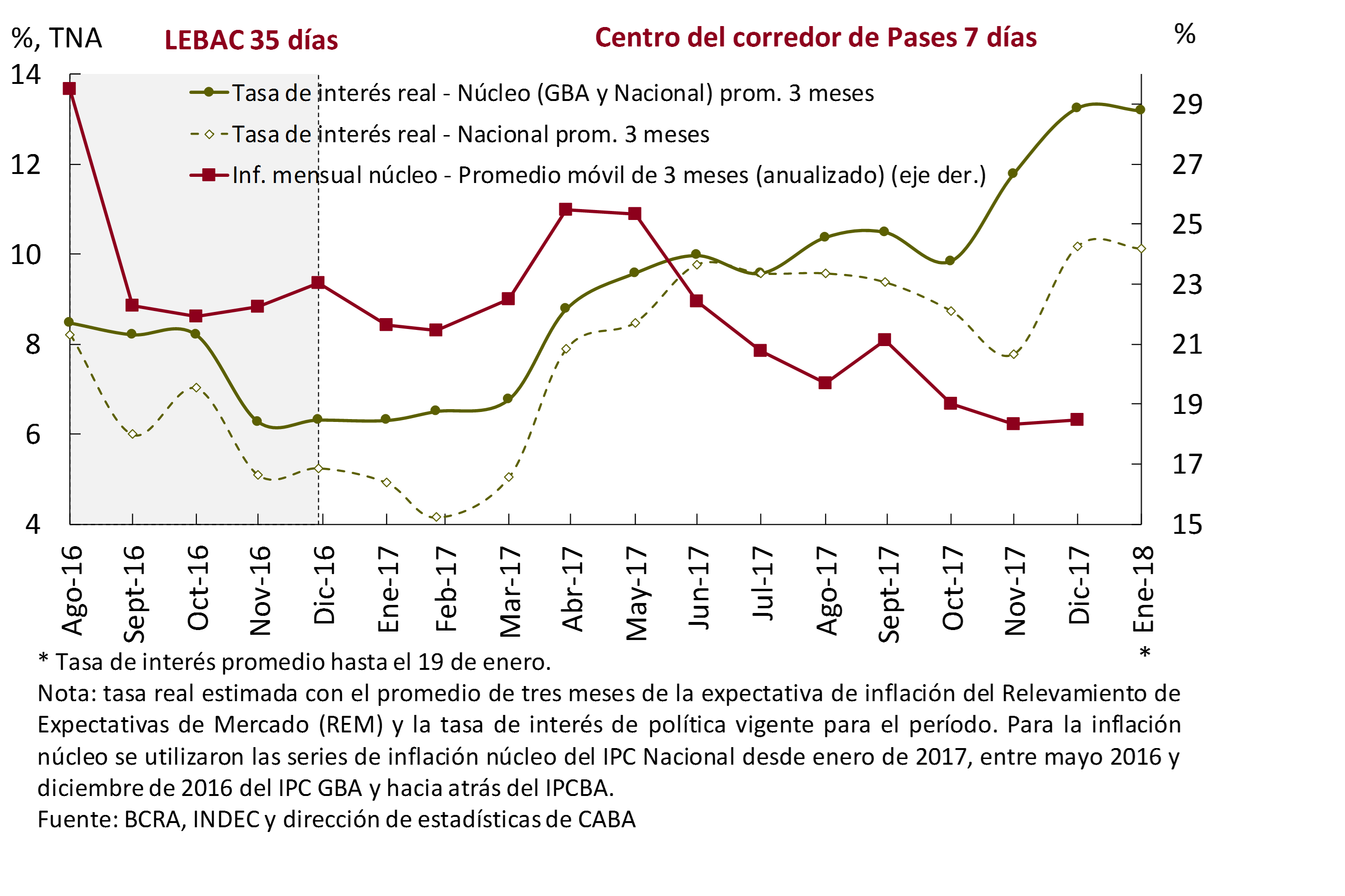
Monetary policy significantly increased its contractionary bias from the second quarter, through both increases in the monetary policy rate and operations in the LEBAC secondary market. Thus, as of May 2017, the economy has returned to the rate of reduction in core inflation foreseen in the January 2017 Monetary Policy Report, breaking the persistence it had been experiencing since 2016 in the second half of the year. However, as the starting point was higher than expected due to the deviation accumulated in the first part of the year, the inflation rate was above the intermediate inflation target set for 2017. Under these conditions, the postponement of the 5% target until 2020, instead of 2019, with intermediate inflation targets of 15% in 2018 and 10% in 2019, implies a path consistent with the pace of disinflation recorded in the second half of 2017.
The continuation of the pace of disinflation for 2018 is benefited by more favourable initial conditions than those of 2017. The contractionary bias of monetary policy is greater with a real interest rate much higher than at the beginning of 2017. An increase in regulated prices of 21.8% is expected, while in 2017 these prices increased 38.7%. Likewise, the gap between inflation, both core and general level, at the end of 2017 and the inflation target is much smaller than at the end of 2016, reducing the challenge presented by inflationary inertia.
Figure 1.2 | Initial conditions: 2017 versus 2018

Considering the pace of disinflation and the set of initial conditions, the BCRA will cautiously adjust the contractionary bias of its monetary policy to achieve its intermediate targets of 15% inflation in 2018, 10% in 2019 and its target of 5% in 2020. In this way, it will promote monetary stability, financial stability, employment and economic development with social equity.
2. International context
The international context impacts Argentina mainly through three channels. Firstly, the level of global activity has a direct impact on our foreign trade and foreign investment flows. Second, the conditions of international credit markets influence the cost of sovereign borrowing and financing of private projects. Finally, the terms of trade impact our foreign trade, affecting wealth and the incentives to produce, consume and invest.
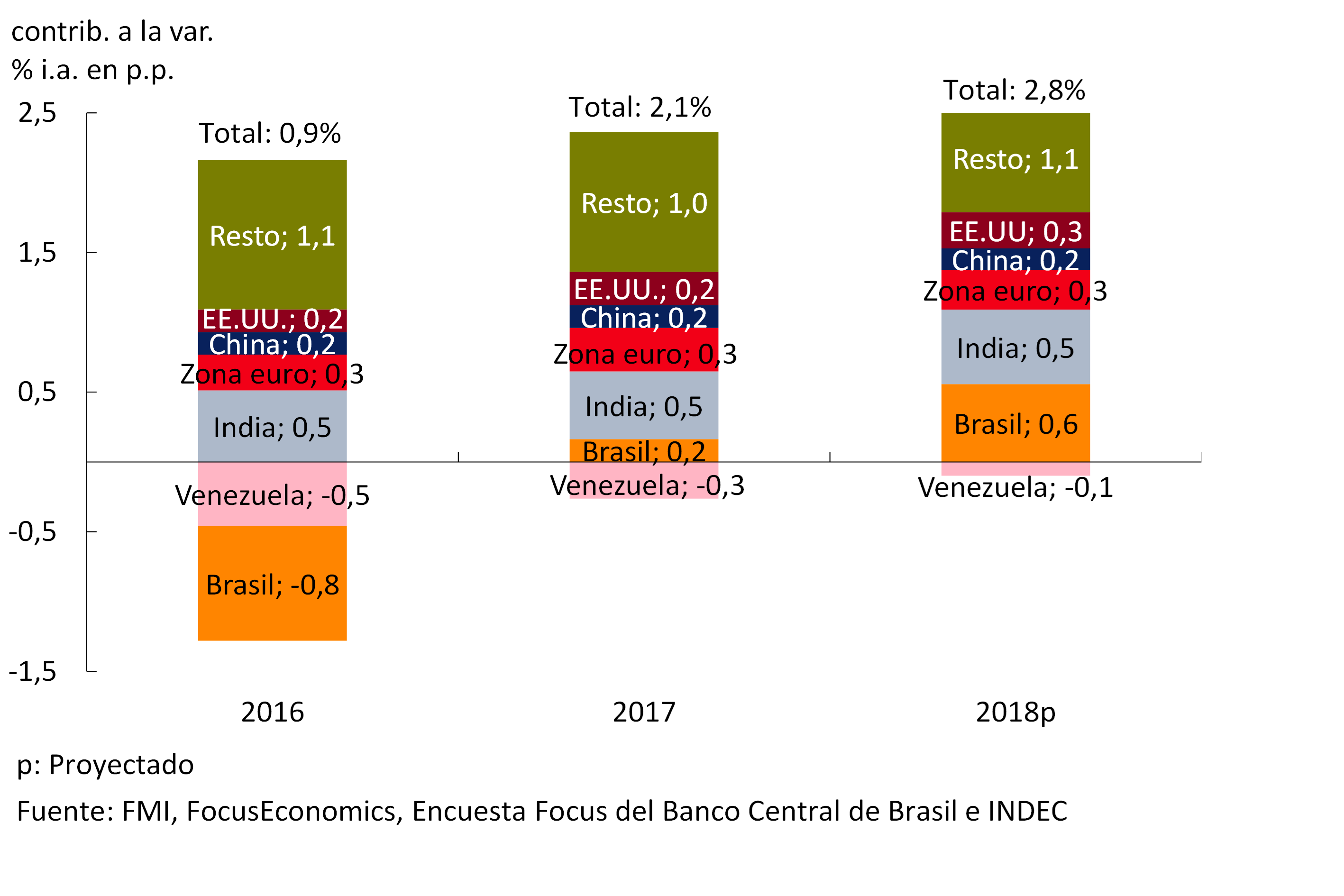
Global economic activity continued to improve in recent months, in both advanced and emerging countries, along with a favorable performance of international financial markets. Projections for 2018 show that this dynamism would continue (see Figure 2.1). In the case of Argentina’s main trading partners, growth accelerated by more than 1 percentage point (p.p.) in 2017 compared to the previous year; and for 2018 an acceleration of 0.7 p.p. is projected, with growth of 2.8% expected. In addition, credit conditions for Argentina continue to be favorable, both for the public sector and for companies, and this is expected to continue during 2018. On the other hand, the prices of Argentina’s main export commodities remained relatively stable in the year, while the multilateral real exchange rate depreciated 0.5% in 2017 (between peaks).
Figure 2.1 | Growth of major trading partners
The prospects of a gradual increase in the U.S. monetary policy rate have so far not affected this favorable scenario. Possible protectionist measures represent a risk to the international real economy. Meanwhile, the greatest source of potential volatility in financial markets seems to be found in possible geopolitical tensions or in the uncertainty associated with electoral processes in Europe and Latin America.
2.1 A higher level of activity is expected in 2018, both globally and for most of our trading partners
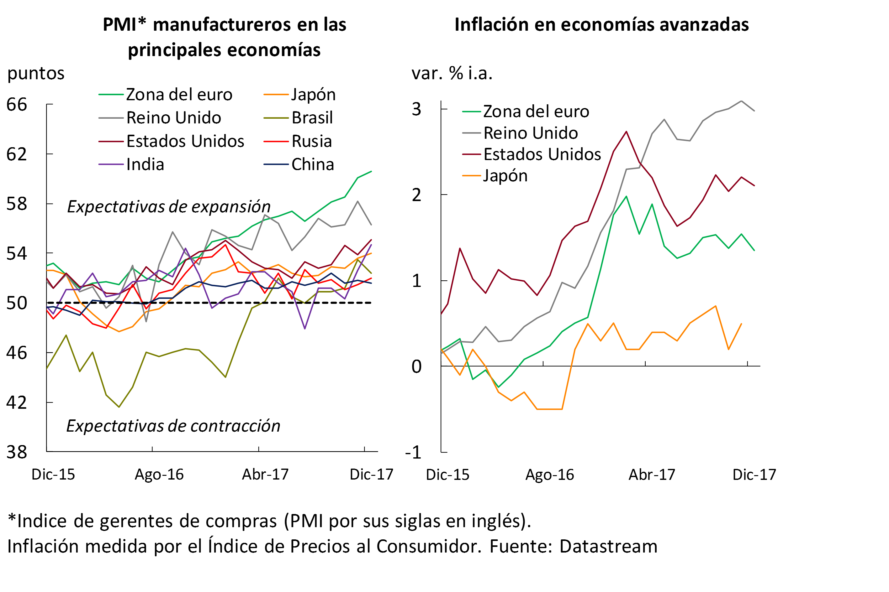
The leading indicators of activity available for the main economies show, in all cases, an expansion, with values mostly higher than those observed in the previous IPOM. On the other hand, according to the most recent data, inflation in 2017 would end up below the highs reached in the year, although with increases in the margin. Thus, inflation in the United States is around target, with inflation in the United Kingdom 1 p.p. above, while in the euro area and Japan it is below (in the latter case, considerably below; see Figure 2.2).
Figure 2.2 | Leading indicators of manufacturing activity and inflation
Brazil, Argentina’s main trading partner and determinant of the region’s economic performance, continues to grow. GDP grew for the third consecutive quarter, having an increase of 0.2% in the July-September period compared to the previous quarter (without seasonality), a lower rate than that of the previous two quarters (0.7% and 1.3%). For its part, the Economic Activity Index prepared by the Central Bank of Brazil (BCB) increased in November by 0.5% compared to the previous month (without seasonality) and by 2.8% year-on-year (see Figure 2.3). In addition, the Industrial Production index increased – also in November – 0.2% compared to the previous month (without seasonality) and 4.6% year-on-year. Finally, with respect to the level of activity, the latest projections of the Focus survey – carried out by the BCB among market analysts – foresee a GDP increase for 2018 of 2.7%, slightly above the 2.5% that was projected at the time of publication of the previous IPOM. The realization of these forecasts would imply a favorable impact on bilateral trade, since the higher growth of Brazilian GDP expected for 2018 would contribute only 0.24 p.p. of growth to Argentine GDP in 2018. 1
Figure 2.3 | Brazil. Macroeconomic indicators
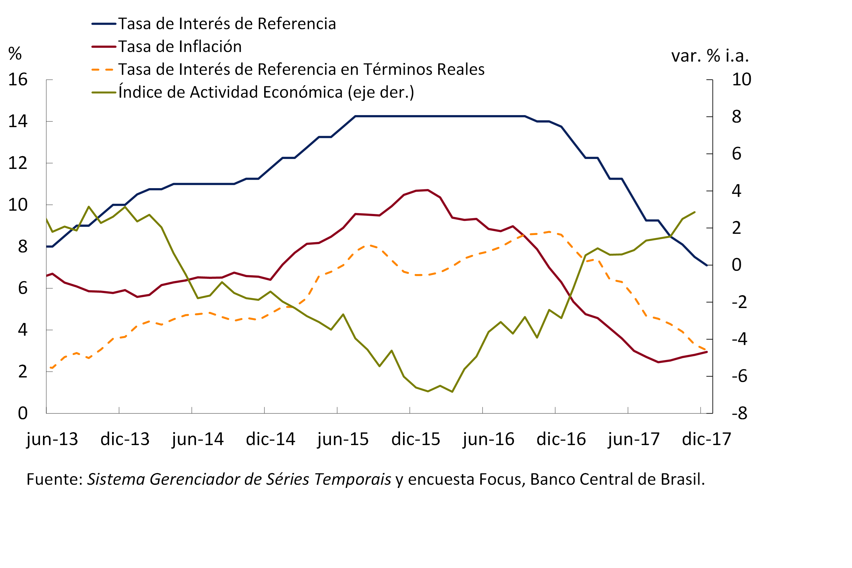
In a context of disinflation, the BCB continued to reduce the monetary policy interest rate (the target on the Selic rate). This decision is linked to the fact that the inflation rate ended 2017 at 2.95%, below the target of 4.5% ± 1.5%. The Selic rate is at 7%, down 125 basis points from its October 2017 value. This resulted in a fall in the monetary policy rate in real terms. According to the Focus survey, virtually no changes are expected from the Selic tax target during 2018.
The euro area, the second destination for Argentine exports, continues to consolidate its economic recovery, according to growth data for the third quarter, leading indicators (see Figure 2.2) and projections for 2018. Seasonally adjusted GDP grew in the third quarter by 0.6% compared to the previous quarter and 2.6% in year-on-year terms. The latest projections of the European Central Bank (ECB) indicate growth of 2.3% and 1.9% for 2018 and 2019, (0.5 p.p. and 0.2 p.p. more than in the previous projection, respectively).
In the euro area, the second destination for Argentine exports, both the growth data for the second quarter and the leading indicators (see Figure 2.2), and the projections for the remainder of the year and 2018 continue to show a consolidation of the recovery. Seasonally adjusted GDP grew by 0.6% in the second quarter compared to the previous quarter. In year-on-year terms, the level of activity increased by 2.1%, the highest rate of change since the first quarter of 2011. For its part, the Purchasing Managers’ Index (PMI) of the manufacturing sector (leading indicator of industrial production) registered in September the highest value since 2011. The IMF’s latest projections show that growth of 2.1% and 1.9% is expected for 2017 and 2018, (0.4 p.p. and 0.3 p.p. more than the previous projection, respectively).
With November’s inflation below the 1.5% target, the ECB did not change its monetary policy interest rate, which remained at the historic low of 0%. The ECB projects an inflation rate of 1.4% for 2018, slightly below the inflation projected for 2017 (1.5%). Despite this, the ECB – at its October monetary policy meeting – reduced the amount of its asset purchase program and extended its operation until September 2018. In this way, the ECB would acquire financial assets for 30,000 million euros per month from January 2018 (half of what it had been buying until then).
The economy of the United States, the third destination for Argentine exports, grew 3.2% (annualized) in the third quarter, above market projections. The unemployment rate (4.1% in December) is at its lowest since late 2000, and below the levels estimated not to accelerate inflation (NAIRU). This happened despite the fact that job creation fell in recent months, as did the participation rate. Regarding growth projections, the Federal Reserve (Fed) increased its estimates for both 2018 and 2019, to 2.5%2 and 2.1% respectively (0.4 p.p. and 0.1 p.p. more than in the projection in force in the previous IPOM).
The Fed’s Monetary Policy Committee announced at its December meeting a further increase in the benchmark interest rate to the range of 1.25-1.5%, as expected. In addition, the same Fed projects further increases of at least 0.75 p.p. during 2018. Finally, the Fed’s balance sheetnormalization program 3 has been operational since October, which in practice implies a less expansive bias of monetary policy, by absorbing liquidity in the market against the sale of securities held by the central bank.
The main destination for Argentina’s primary commodity exports, China, is expected to end 2017 with a year-on-year GDP growth of 6.8%, driven mainly by private consumption and investment. It is noteworthy that the dynamism of imports continued in recent months, since in October they had a year-on-year growth of 18.7%, partly driven by an appreciation of the yuan against the US dollar of 6.3% in 2017. Finally, lower GDP growth is expected for 2018, at around 6.6%, mainly due to lower export growth.
2.2 Favorable credit conditions for Argentina would continue in 2018
Since the last IPOM, three central banks that in recent years had carried out a strongly expansive monetary policy have taken measures to reduce this stimulus. The Fed and ECB have begun to reduce unconventional monetary stimulus, although the former is further along in the process. Alongside them, the Bank of England (BoE) took measures with a contractionary monetary bias for the first time in more than ten years. For its part, the Bank of Japan (BoJ) is continuing with its quantitative easing program, although it could start tapering this program in 2018. Despite the recent measures by the Fed, the ECB and the BoE, the large monetary expansion of the last decade allows us to expect that global liquidity conditions will continue to be accommodative for emerging countries. This would allow Argentina to continue financing itself on favourable terms.
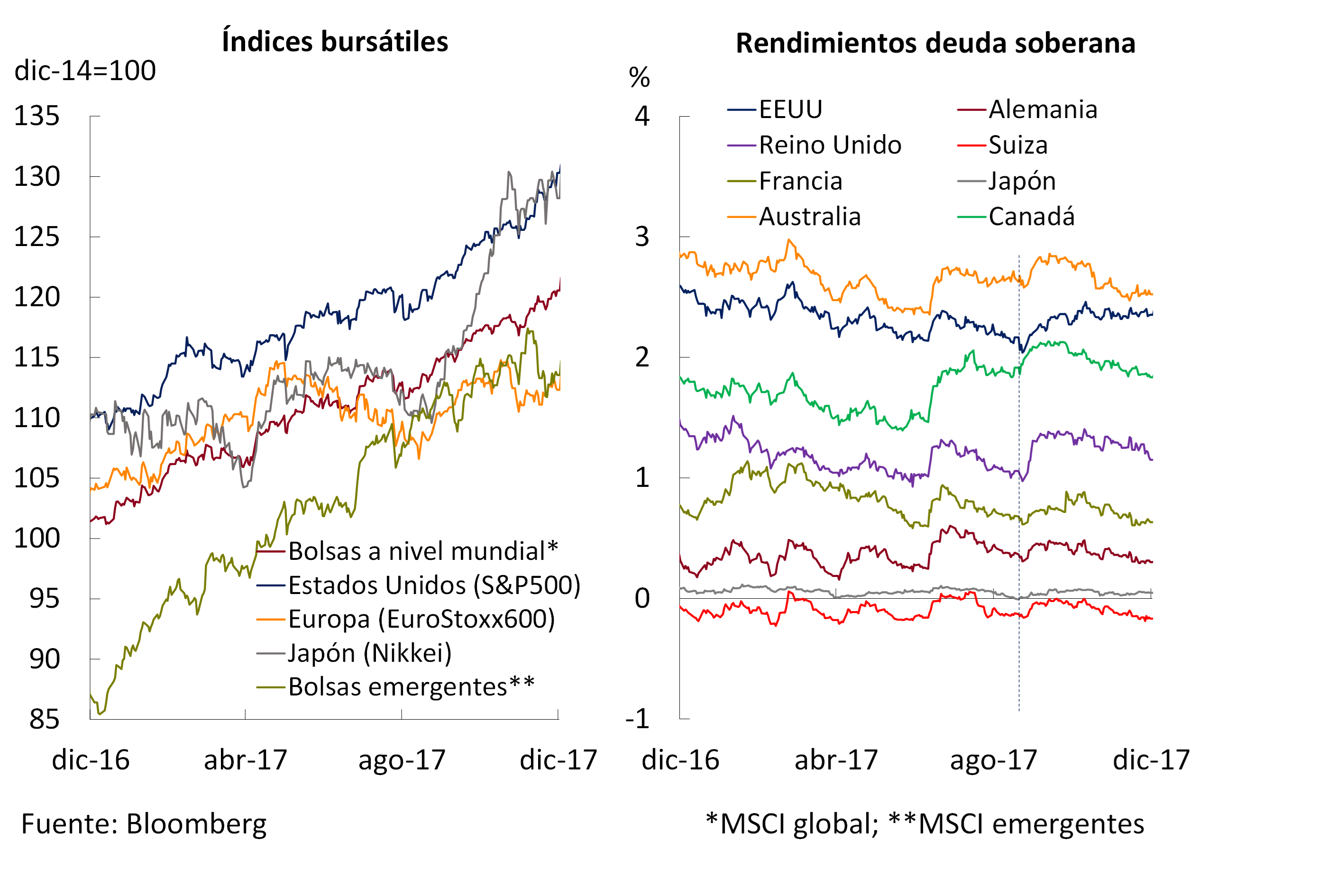
International financial markets continued to be generally bullish and less volatile for both equity and fixed income assets (see Figure 2.4). Stock indices maintained their upward trend throughout 2017, in some cases reaching all-time highs, as in the case of the S&P500, or the highest in the last 25 years, as in the case of the Nikkei. The yields on government debt securities of most developed countries had a declining trend throughout 2017 that began to reverse in September, after the Fed’s announcement of the beginning of its balance sheet normalization policy. However, they ended 2017 with a lower performance than a year ago (average of December 2017 compared to December 2016).
Figure 2.4 | stock indices and 10-year sovereign bond yields
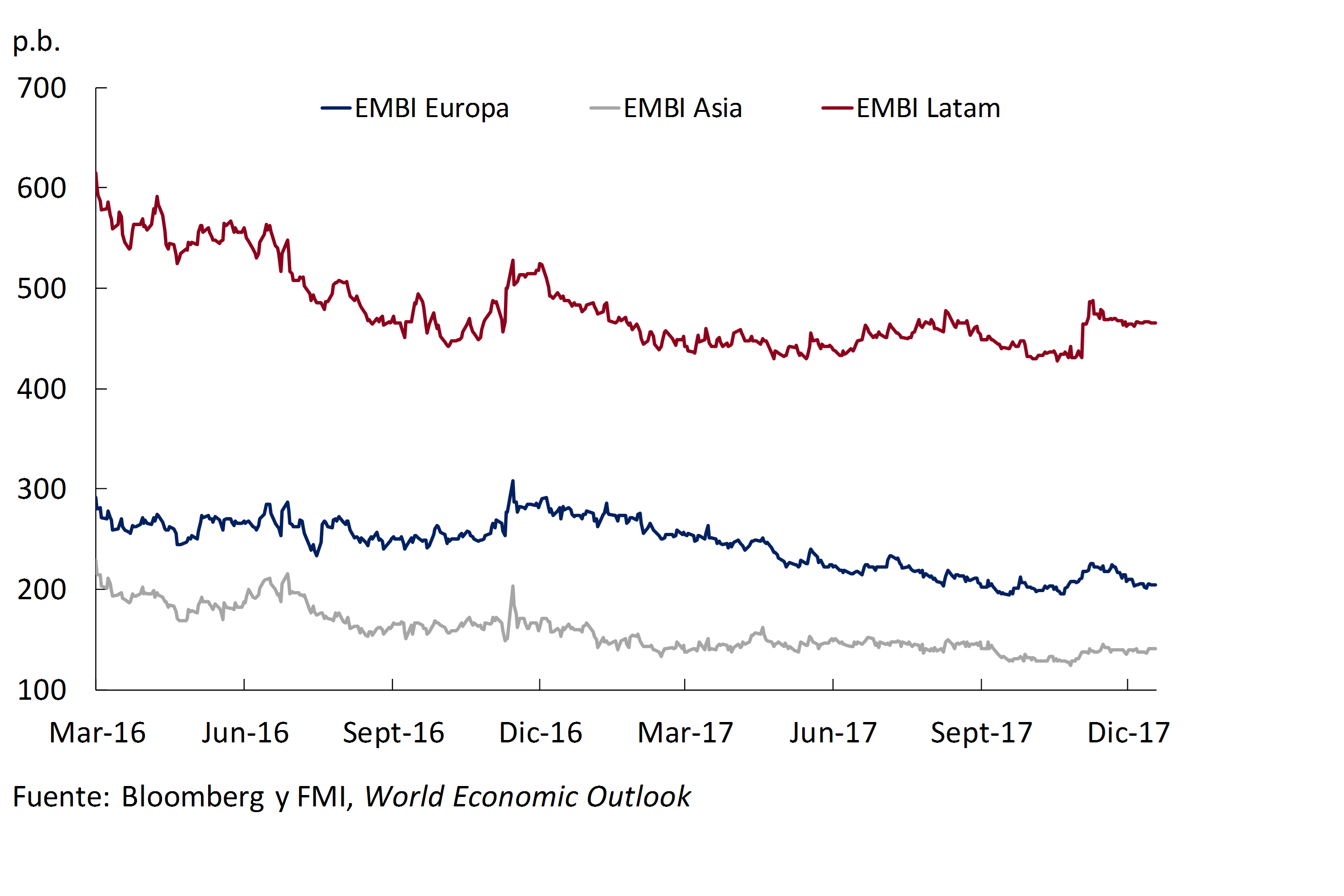
During the year, the sovereign risk premiums of emerging countries also fell. Since the Fed’s September announcement, they have tended to rise, particularly in the case of Latin America (see Figure 2.5).
Figure 2.5 | Emerging. Sovereign risk premiums
The total amount of debt issuances of emerging countries in international markets (sovereign and corporate debt), measured in gross terms, increased by 38% YoY in 2017, with an increase in the participation of the corporate sector. In the case of Argentina, the gross amount of placements in international markets increased by 7%; it was 6% in the case of the national non-financial public sector (NFPS, excluding from the calculation the 2016 issuances linked to the restructuring of debt in default) and 11% in the corporate sector. At the beginning of 2018, the NFPS placed debt for approximately US$ 9,000 million.
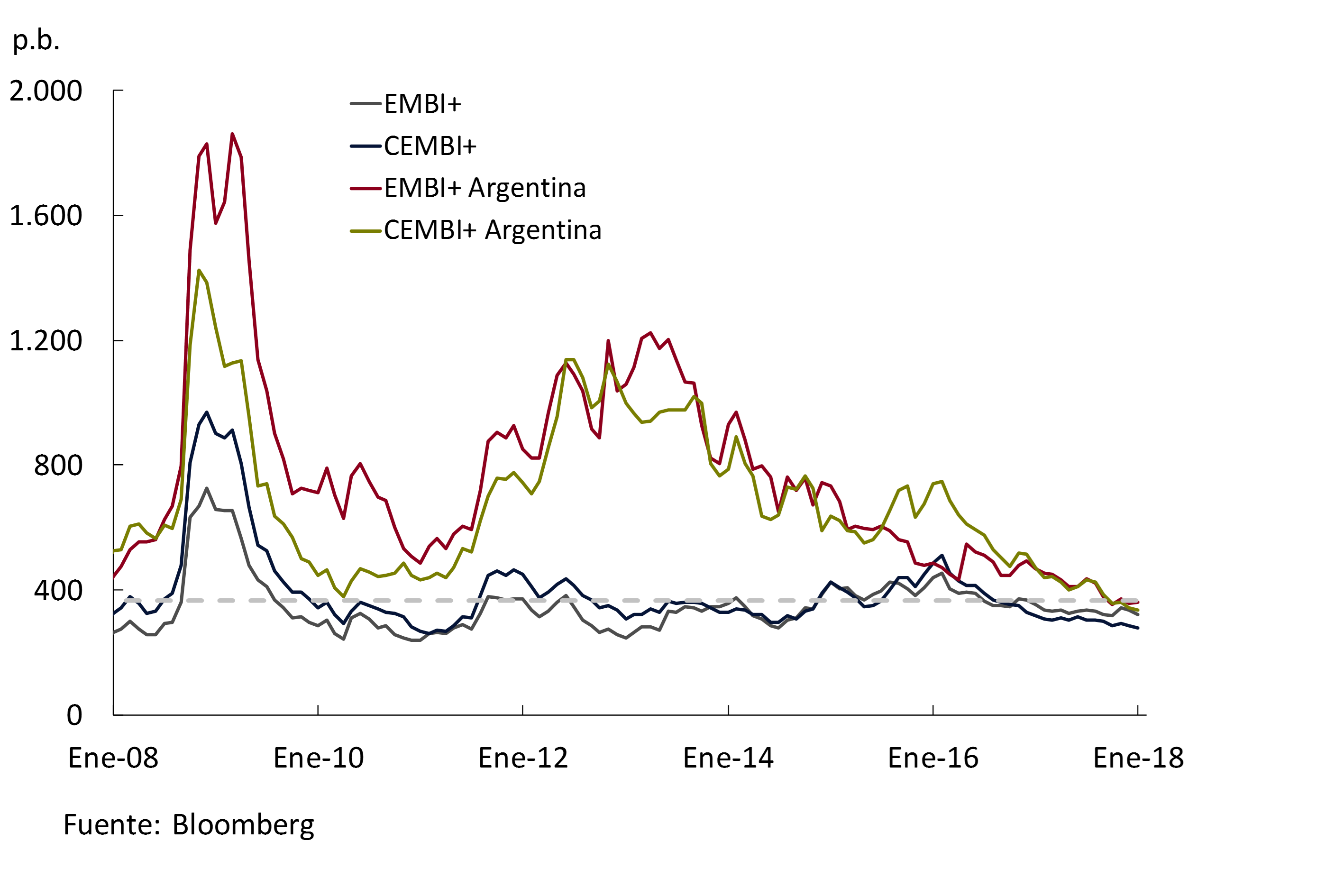
For Argentina, credit conditions improved even more than for the rest of the emerging economies, placing the Argentine country risk at around 360 bp for the EMBI+ Argentina index (almost unchanged from the previous IPOM), and at 356 bp for the CEMBI+ Argentina, slightly below October, both values being the lowest in the last ten years (see Figure 2.6). In this way, the public sector and Argentine companies are financing themselves at lower interest rates in international markets.
Figure 2.6 | Sovereign and corporate debt risk indicators
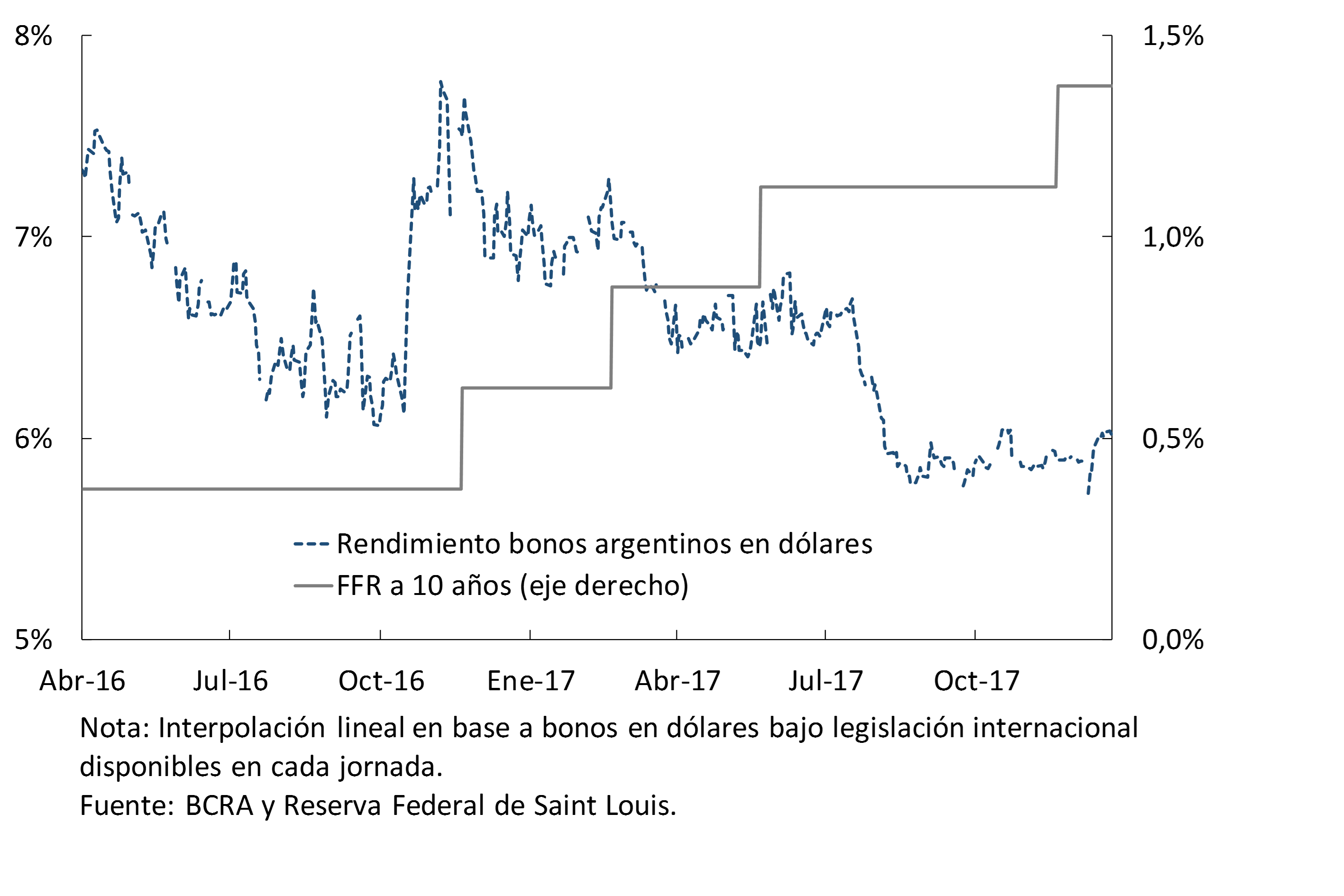
At this point, it is worth clarifying that the expected increases in the Federal Funds rate for 2018 would have a negative impact on the external financing conditions faced by Argentina; but this effect can be counteracted if the risk premiums of Argentine securities continue to fall, as they have done since 2016 (See Figure 2.7). In fact, if the EMBI index for Argentina is compared with those of countries such as Brazil, Colombia or Mexico, for example, it is observed that the cost of external financing can still be significantly reduced.
Figure 2.7 | Cost of external borrowing and the Federal Reserve’s monetary policy interest rate
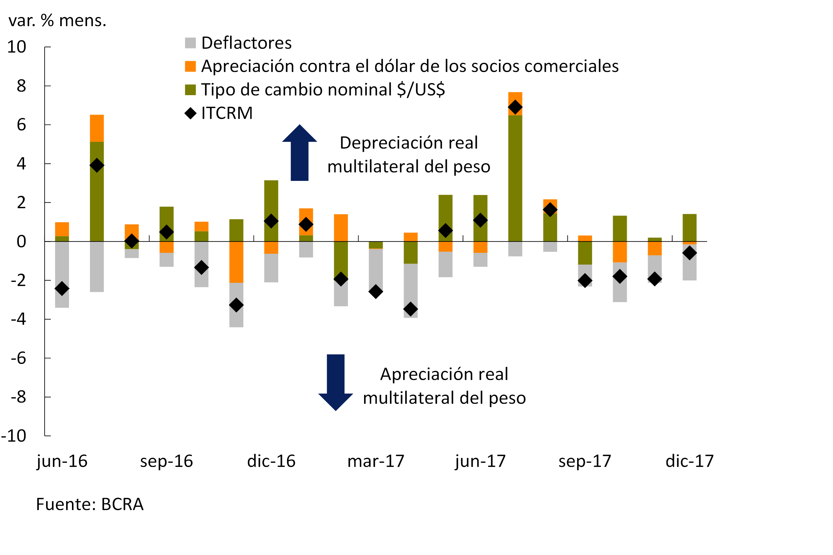
The Multilateral Real Exchange Rate Index (ITCRM) appreciated 4.1% in the quarter, driven both by the depreciation of the currencies of our trading partners against the dollar by 1.0%, as well as by the higher relative inflation in Argentina; this was partly offset by the nominal depreciation of the peso against the dollar (1.6%; see Figure 2.8).
Figure 2.8 | ITCRM variation by component
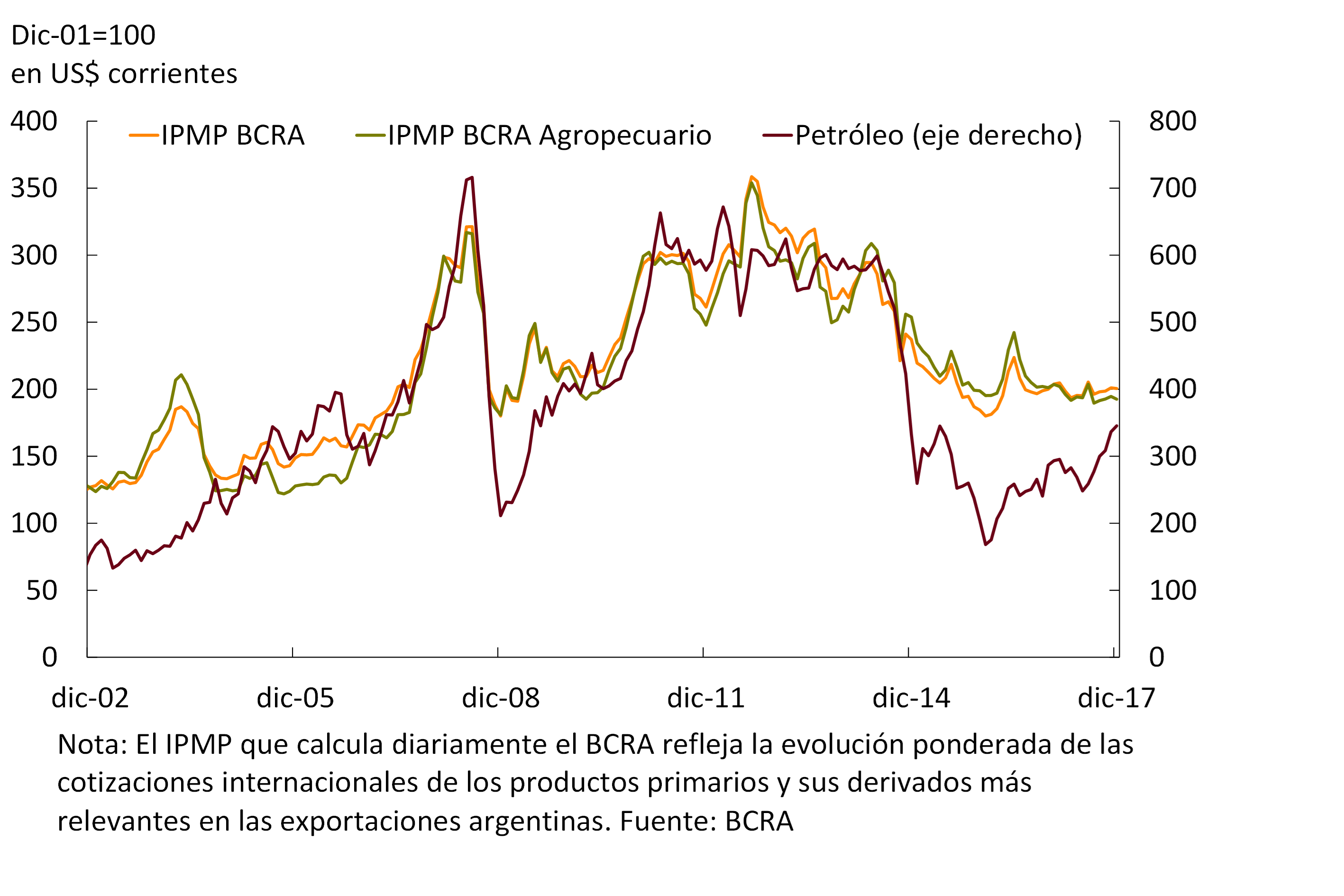
The prices of primary goods continue to evolve unevenly between those related to oil and the rest. The upward trend in the price of oil that began in the middle of last year continued, with a cumulative increase of 44%. Meanwhile, the Commodity Price Index (CPMP BCRA) – which reflects the evolution of Argentina’s main export commodities, with a marked influence on the local economic cycle – remained relatively stable in recent months (0.3% year-on-year variation in December). The BCRA agricultural IPMP moderated the downward trend of recent months (-21% in December compared to June 2016) (see Figure 2.9), partly thanks to an increase in the price of soybeans in the last months of the year.
Figure 2.9 | International commodity prices
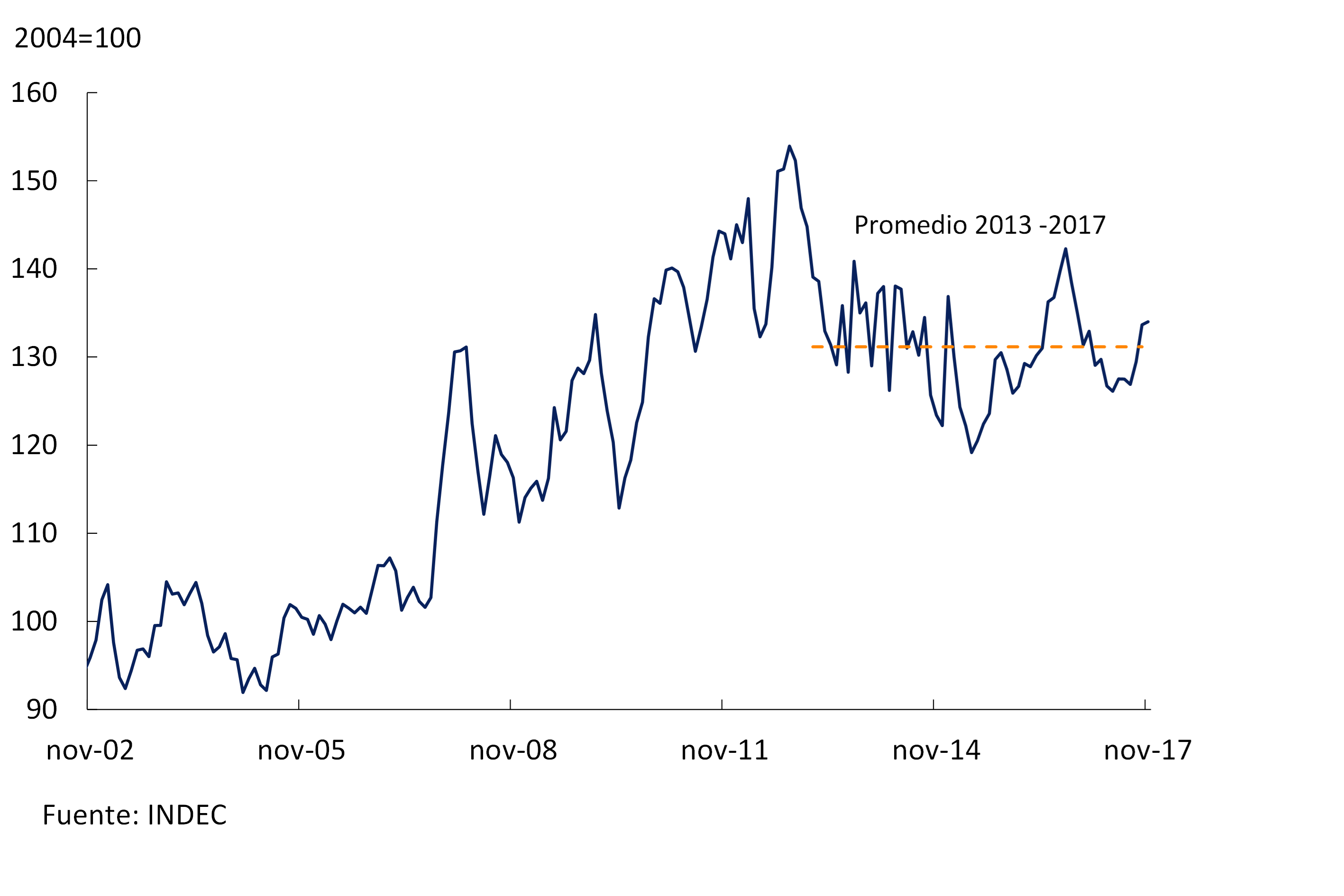
Finally, the terms of trade (quotient between the prices of Argentine exports and imports)4 were much of 2017 below the 2013-2017 average. In the last quarter of the year they seem to be recovering (with data up to November; see Figure 2.10).
Figure 2.10 | Terms of Trade Index
In summary, an improvement in global economic activity is expected in the coming months, especially in the case of our trading partners. This would have a favorable impact on the demand for Argentine exports. In addition, conditions of abundant liquidity for emerging countries are expected to continue in 2018, despite the tightening of monetary policy by some central banks in advanced countries. Therefore, credit conditions for Argentina are expected to remain favorable.
3. Economic activity
The economy achieved a year and a half of uninterrupted growth, constituting the longest expansion phase since the period 2009-2011. Policies aimed at correcting macroeconomic imbalances and structural reforms have allowed growth during 2017 at a sustained rate of 4% annualized with low volatility. Investment continues to play a leading role, private consumption is slightly above its trend and public consumption is slowing down. At the sectoral level, the expansion is widespread and accompanied by increases in productivity in most sectors. At the same time, the real exchange rate has remained stable under a floating exchange rate regime and real wages have grown. The BCRA expects sustained growth to continue with less volatility in the cycle, leaving behind the stage of output stagnation. This view is shared by the participants of the Market Expectations Survey (REM), who projected that the economy will continue to expand annually by around 3% in 2018 and 2019.
3.1 The economy completed a year and a half of uninterrupted growth
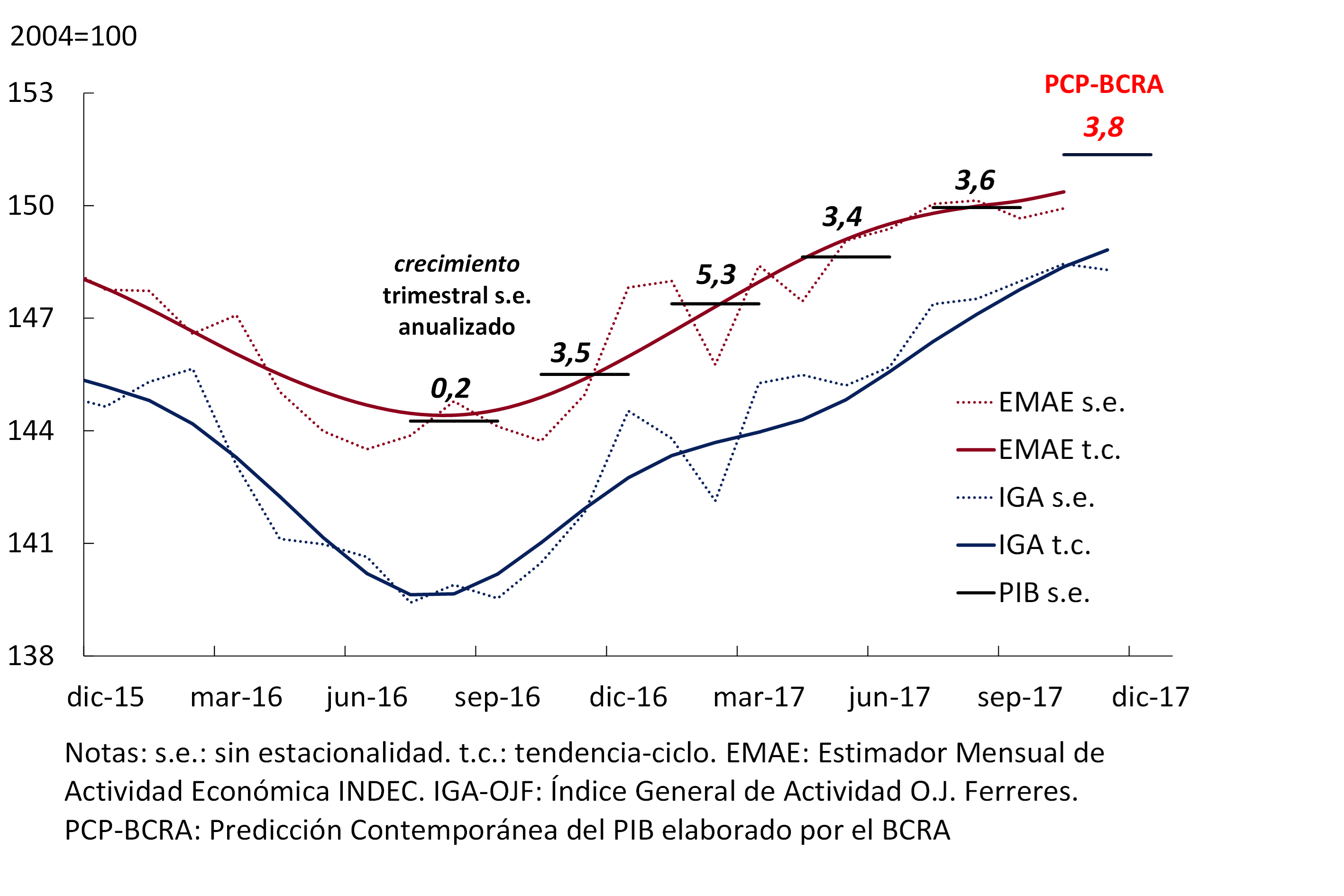
During the fourth quarter of 2017, the economy completed six quarters of uninterrupted growth with a reduction in volatility. The latest BCRA Contemporary GDP Prediction (PCP-BCRA) indicates a quarterly increase of 0.94% without seasonality (s.e.), while the forecast of REM analysts is 1% s.e.5 Thus, GDP would have expanded at an average annualized quarterly rate of close to 4% during 2017 (see Figure 3.1).
Figure 3.1 | Evolution of economic activity
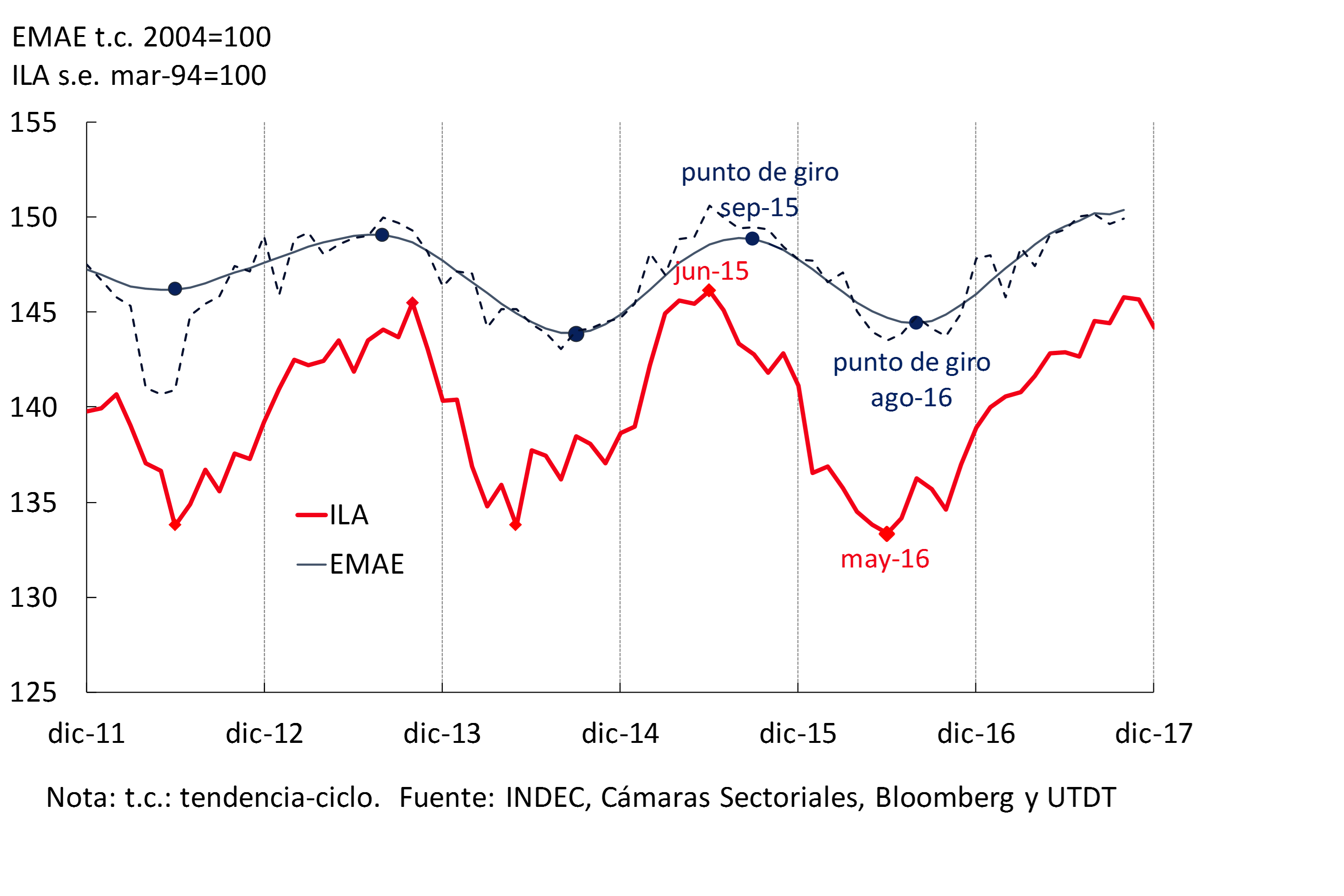
Although the Leading Activity Indicator (ILA) prepared by the BCRA showed a fall in December, this indicator continues to anticipate that the expansionary cycle will continue in the coming months6 (see Figure 3.2).
Figure 3.2 | Leading Activity Indicator
3.1.1 Domestic demand expands above GDP, at rates above 5% per year
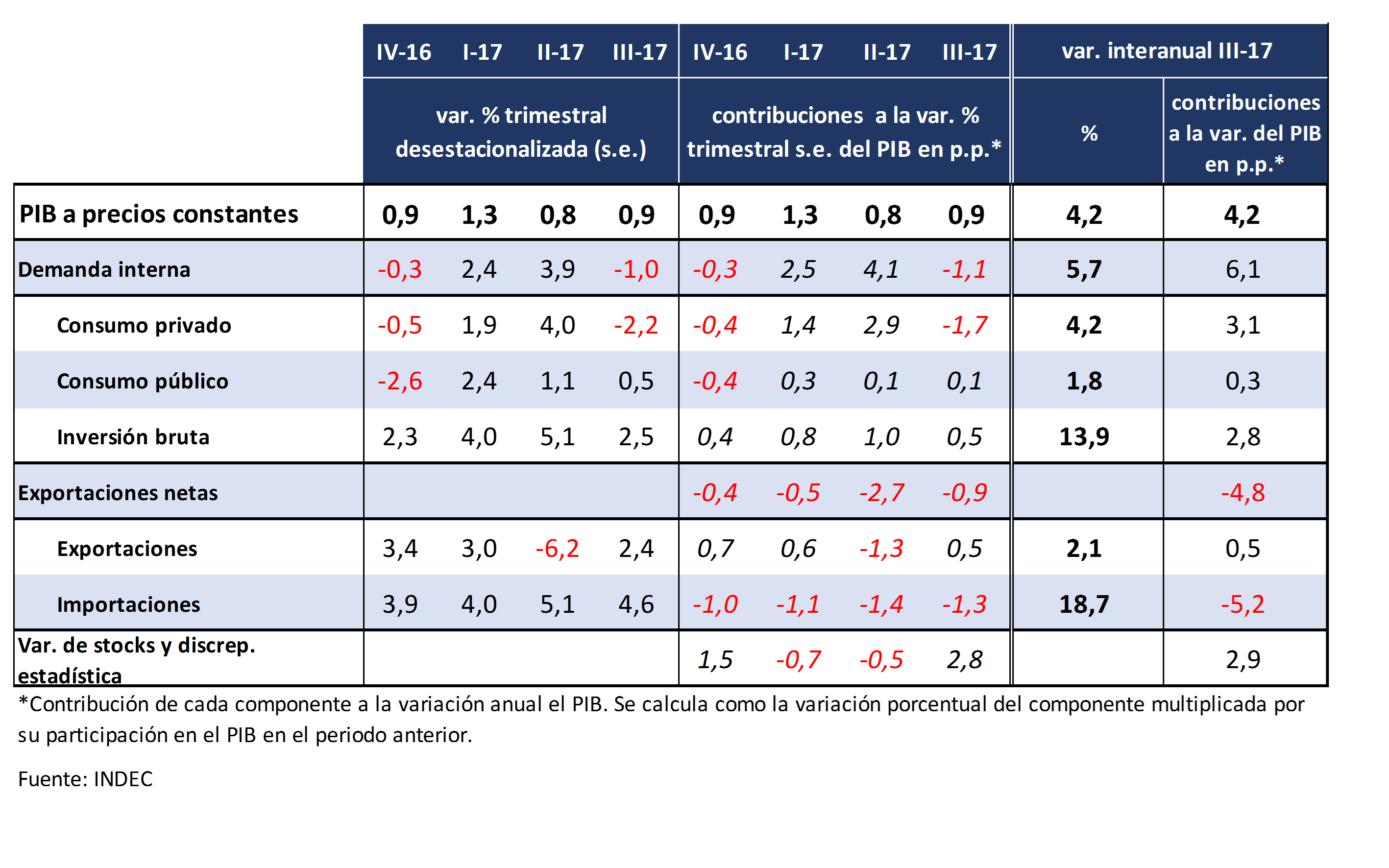
In the third quarter, domestic demand (investment and total consumption) grew at a year-on-year rate of 5.7%, with a notable increase in investment (13.9% YoY), with a high share of the imported component (see Table 3.1).
Table 3.1 | GDP growth and contributions of its components
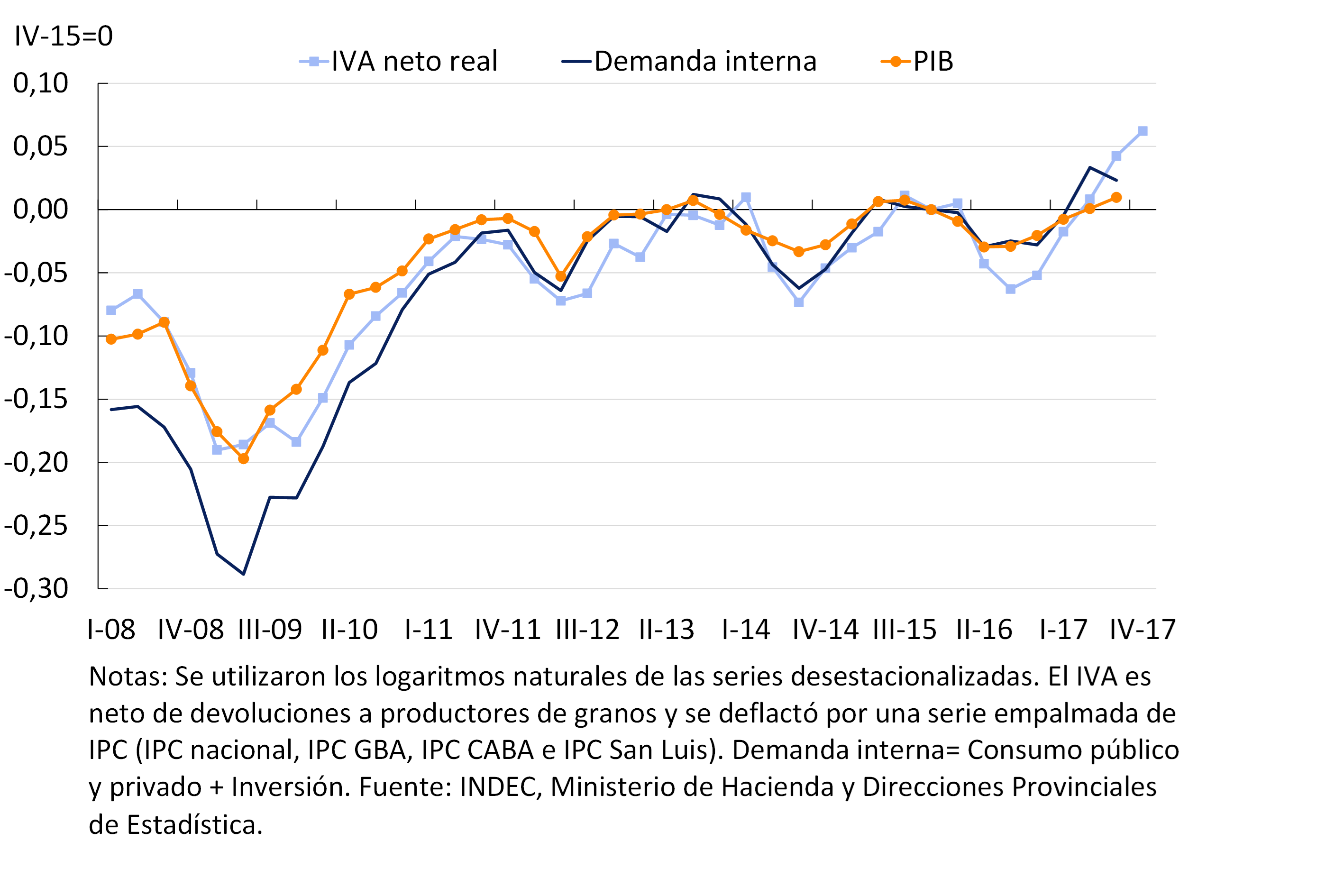
Different partial indicators suggest that domestic demand continued to increase in the last quarter of last year. Gross VAT collection deflated by national CPI (net of refunds to grain producers) rose 2.0% quarter-on-quarter (see Figure 3.3). Imported quantities directly linked to consumption and investment increased 1.1% s.e. in the October-November two-month period compared to the previous quarter. Personal and credit card loans grew 2.2% s.e. quarter-on-quarter in real terms.
Figure 3.3 | Real VAT Collection, Domestic Demand, and GDP
3.1.2 Investment consolidates its leading role in growth
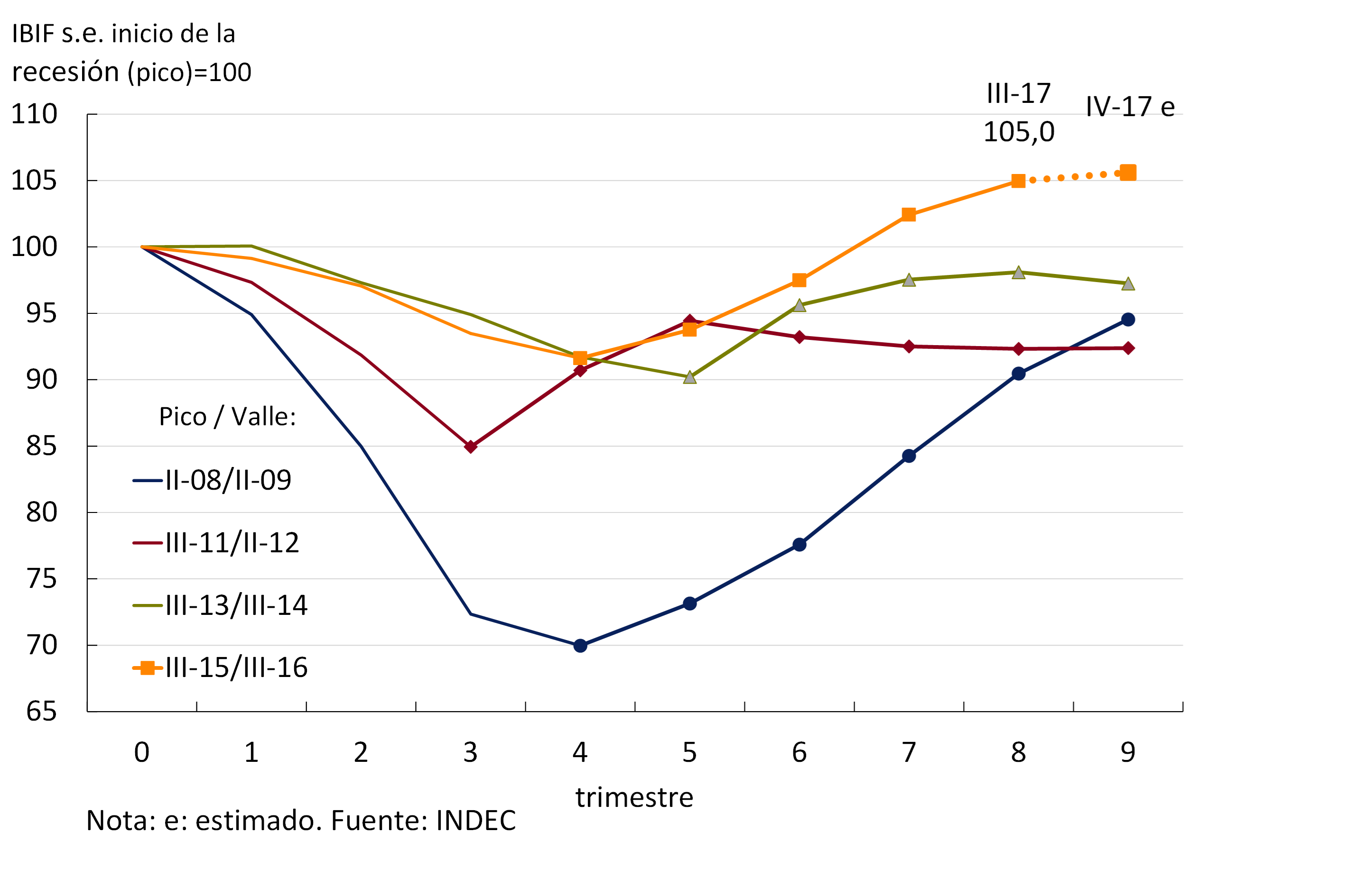
In line with what was anticipated in the previous IPOM, gross domestic fixed investment (GDI) increased for the fourth consecutive time in the third quarter of 2017, and did so at an average annualized rate of 14.6%. The leading indicators—sales volume of domestic and imported equipment and the evolution of construction activity—allow us to anticipate a new increase in the fourth quarter of the year, remaining clearly above the levels corresponding to other economic recoveries in recent history (see Chart 3.4).
Figure 3.4 | Investment performance in recent recoveries
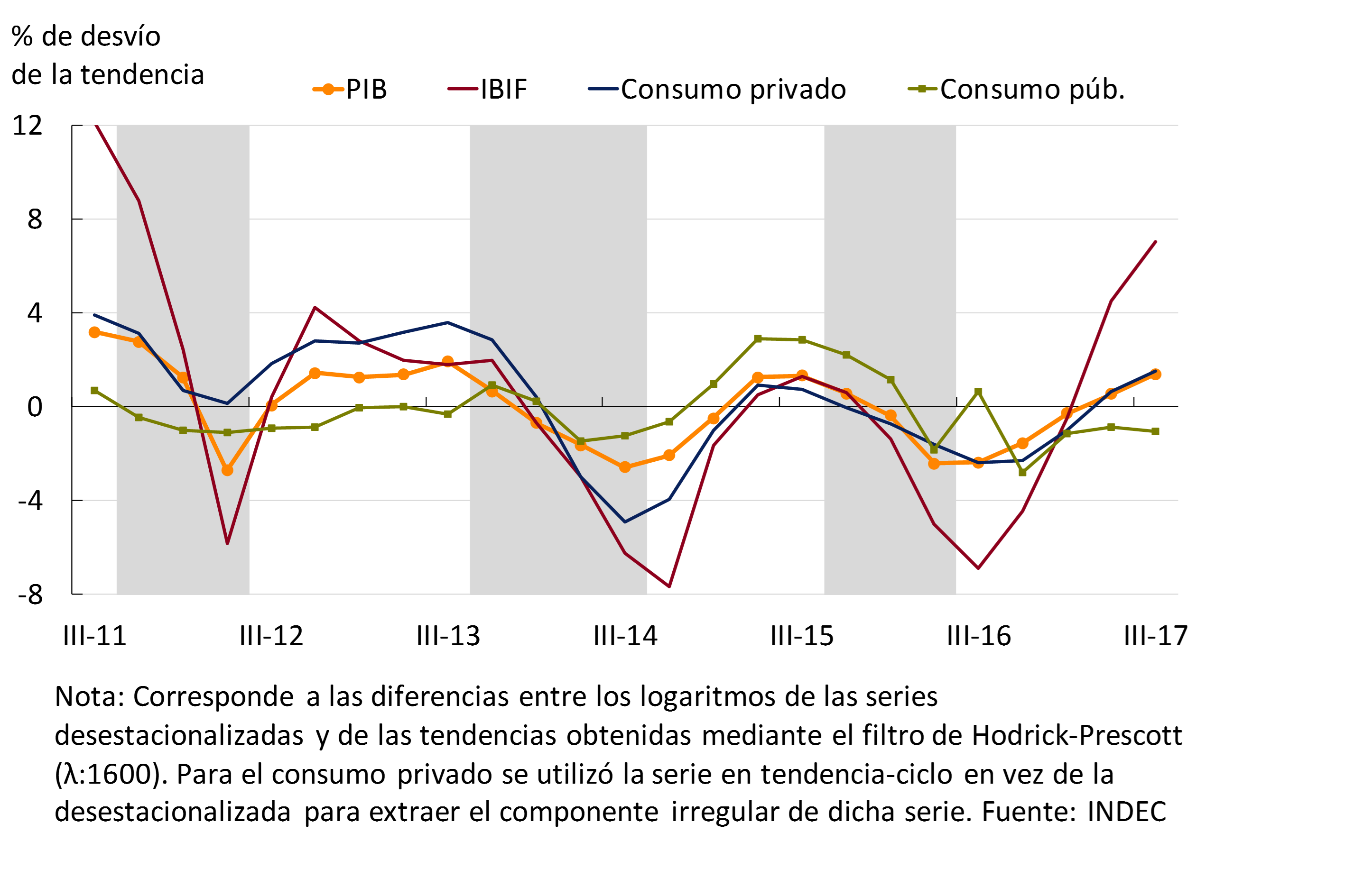
Investment is now the component of aggregate spending with the greatest traction on the output cycle, unlike previous cyclical recoveries where the main driver was public or private consumption (see Figure 3.5).
Figure 3.5 | Cyclical behaviour of GDP, investment and consumption
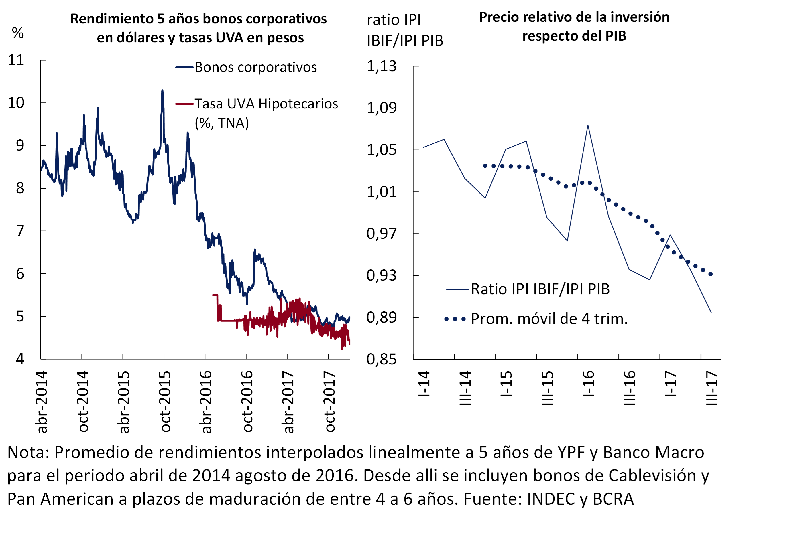
From 2016 onwards, IBIF responded positively to the elimination of distortions and correction of macroeconomic imbalances. The fall in investment costs together with the expectation of increases in productivity boosted the expansionary investment cycle (see Figure 3.6). The first is related to a fall in the relative price of capital and the reduction in interest rates faced by the public and private sectors in international markets. Thus, investment left behind four years of stagnation.
Figure 3.6 | Return, rates and relative price of the investment
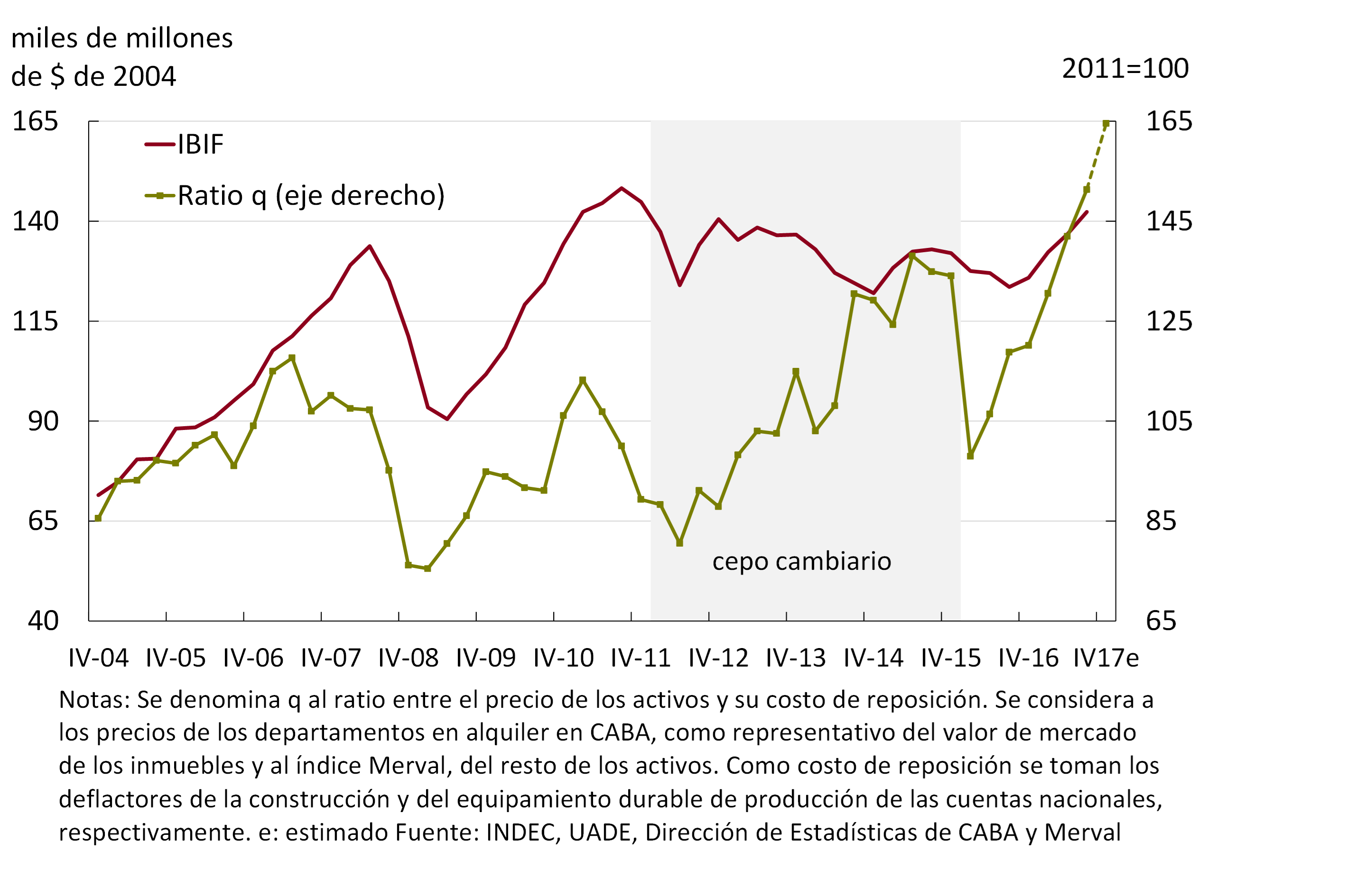
This improvement in investment can be anticipated by Tobin’s Q ratio, which relates the market value of the invested assets to their replacement cost. During the period 2004-2017, it is verified that when the Q ratio rises, investment responds positively and vice versa, with the exception of the period 2013-2015, which is atypical, when there is an increase in the market value of the assets with respect to the replacement cost without a positive response from the investment. This could be interpreted as evidence of the impacts of exchange restrictions (cepo) and the expectation of economic reforms that would improve the business climate. This market optimism did not translate into an increase in investment until the macroeconomic reorganization took place. The strong increase in the Q-ratio during 2017 suggests that investment will continue to show positive dynamics in the coming months (see Figure 3.7).
Figure 3.7 | Investment and ratio of market value to cost of assets
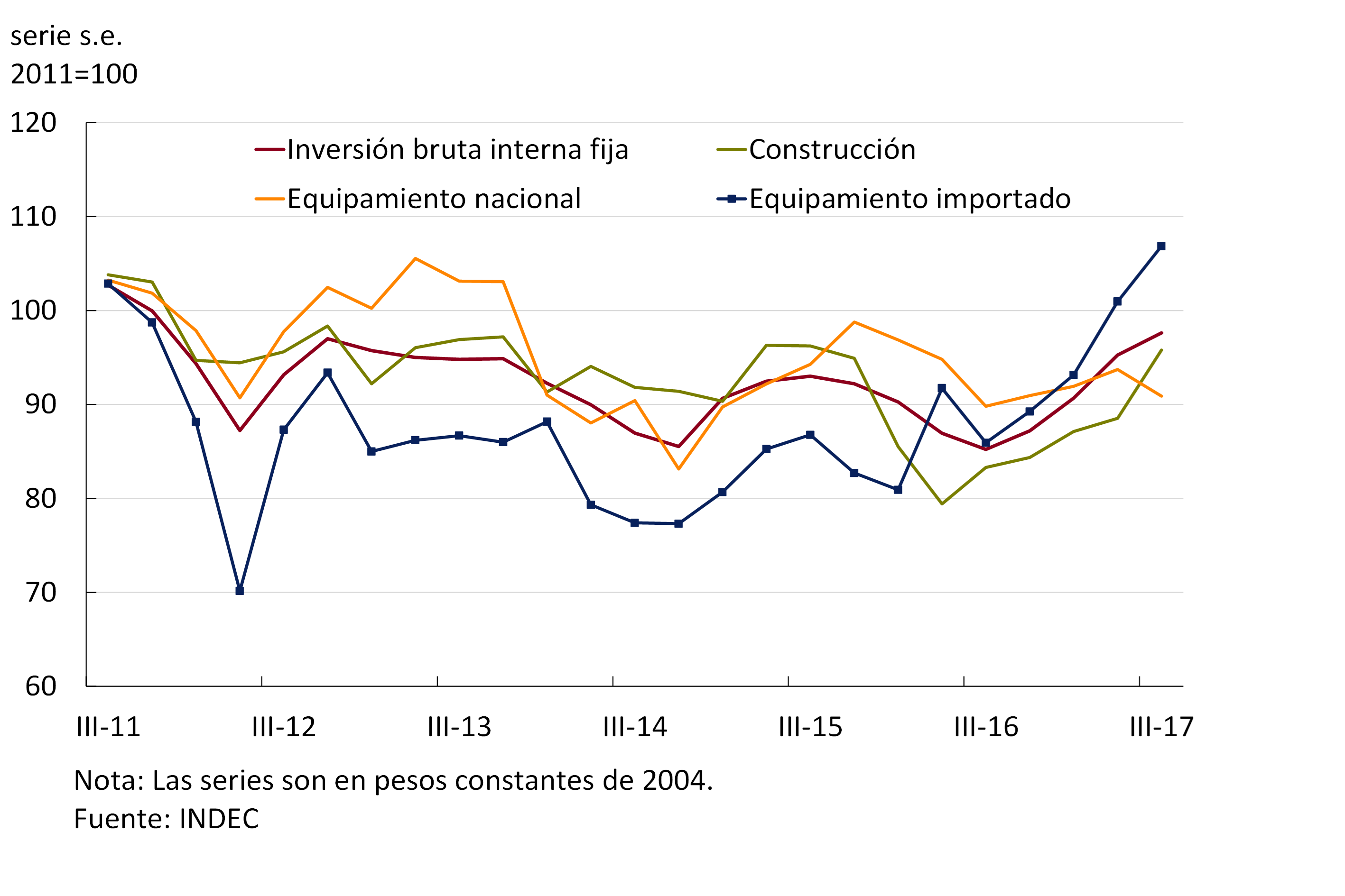
The growth in investment in the third quarter of 2017 was due to the combined increase in construction (14.7% YoY in the third quarter) and durable equipment (15% YoY).7, with a strong incidence of expenditure on machinery and equipment of imported origin (30.3% YoY) which, measured at 2004 prices, reached a maximum of 35.4% participation in the IBIF (see Figure 3.8).
Figure 3.8 | Evolution of investment components
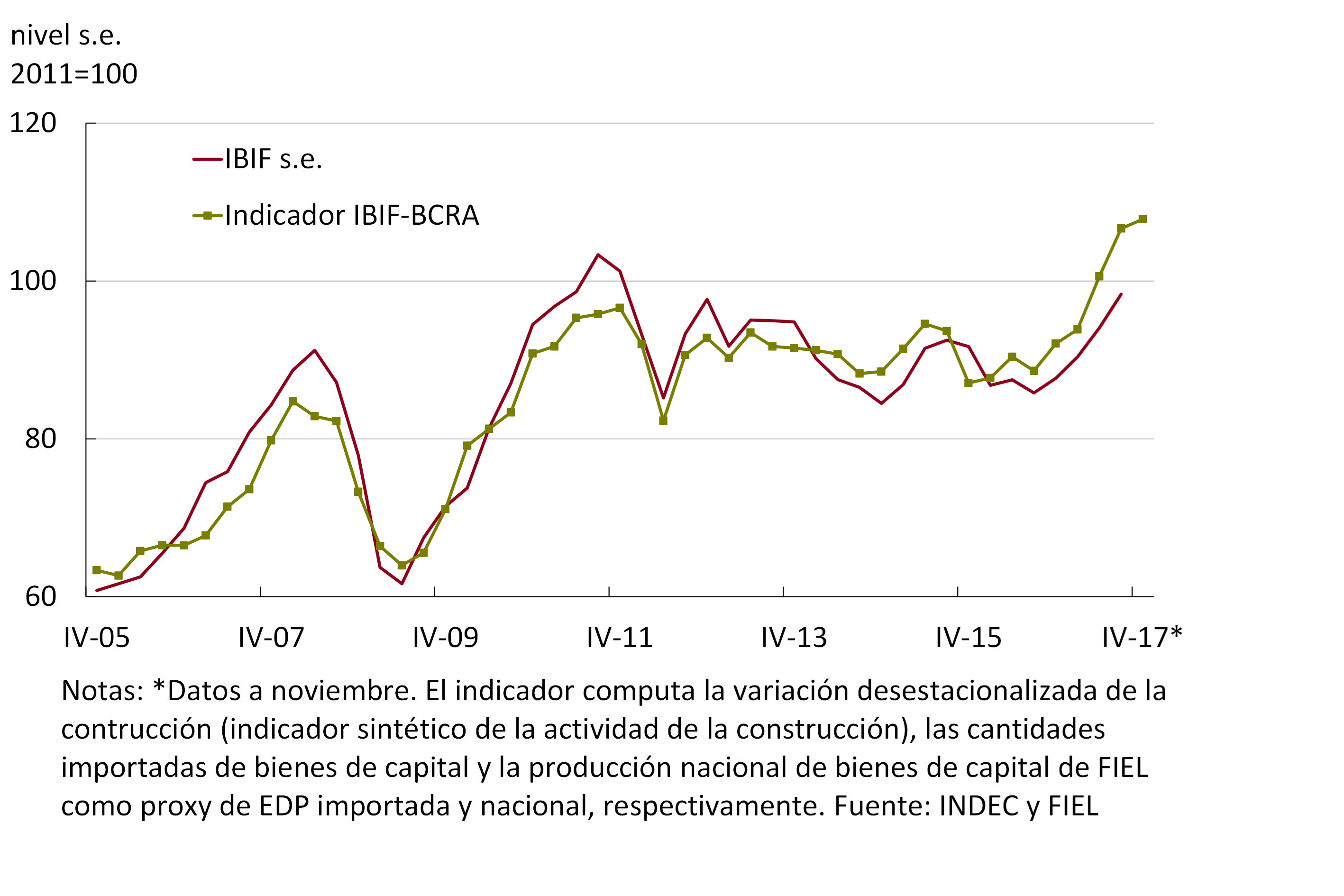
In the last quarter of 2017, leading indicators indicate that the upward trajectory of investment would have continued. The IBIF-BCRA8 indicator, whose variation is a weighted average of the variations of the leading indicators, increased 1.1% quarter-on-quarter s.e. (17.1% y.o.y.). In the same sense, the Coincident Investment Index prepared by the Ministry of Finance registered a rise of 16.4% y.o.y. Thus, investment growth in 2017 would have been the highest in the last six years (see Figure 3.9).
Figure 3.9 | Investment evolution
Box. Foreign Investments in Argentina
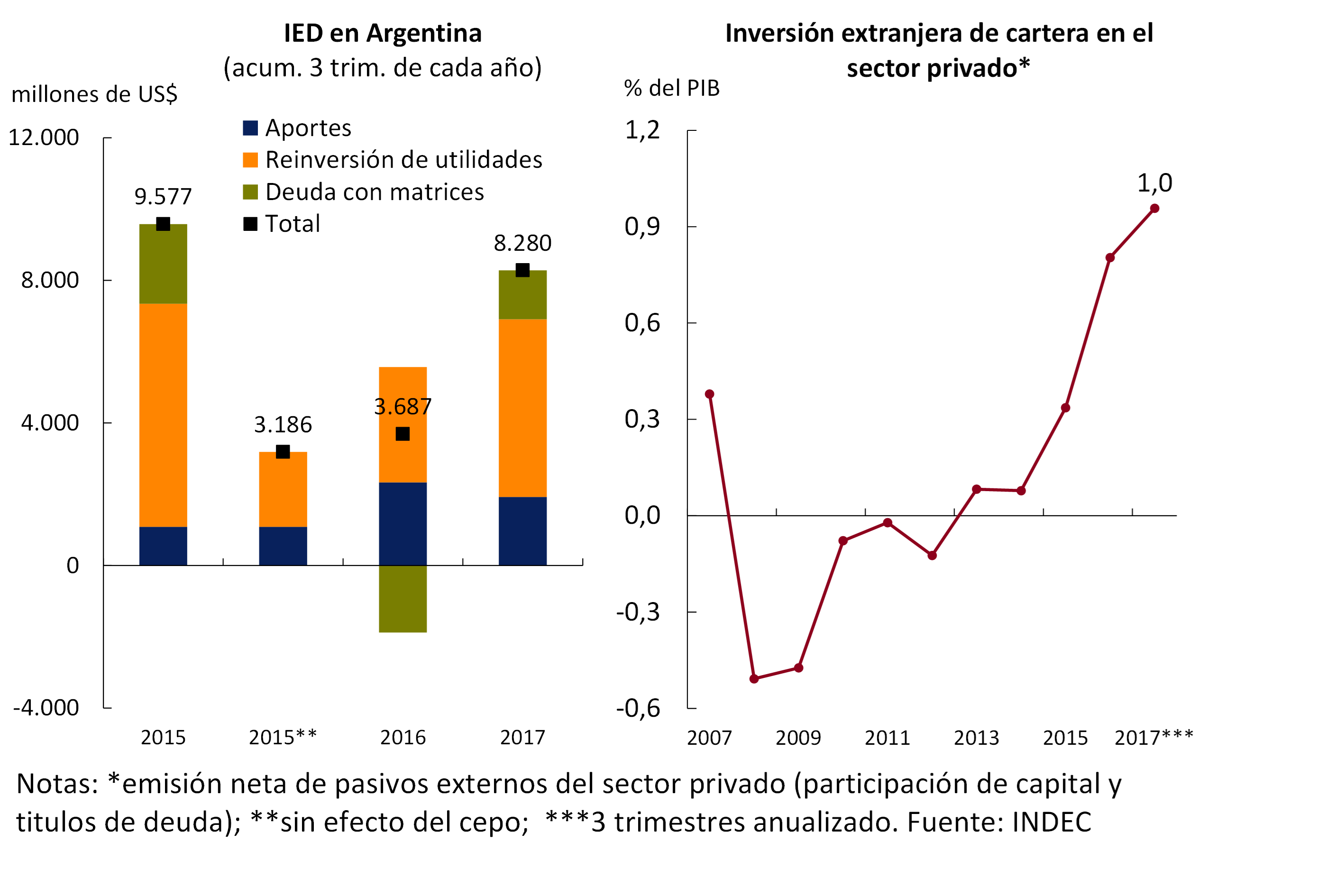
Inflows of foreign direct investment (FDI) to Argentina stood at around US$ 8,300 million in the first three quarters of 2017, US$ 4,593 million higher than those registered in the same period of 2016. However, throughout 2016 firms normalized their relationship with parent companies, which implied a reduction in the stock of commercial debt, as well as a greater remittance of retained earnings during the period 2012-2015 (see Figure 3.10).
The level of FDI in 2017 is lower than that recorded in 2015 because at that time the investment decisions of firms were conditioned by the validity of exchange restrictions. If in 2015 firms had been able to transfer to their parent companies a percentage of their earnings similar to those of the 2004/2011 period and had not been forced to increase their commercial debt, the FDI flow in 2015 would have been around US$3,200 million, a level substantially lower than that observed in 2017.
Since the lifting of the clamps, capital contributions remained at levels higher than those of the previous period: from about US$1,100 million in the first three quarters of 2015 to about US$2,300 million and US$2,000 million in the same period of 2016 and 2017, respectively.
The new rules of the game in force since December 2015 – which allowed firms to access international credit markets again – also had an impact on portfolio investment flows in the private sector (net issuance of external liabilities for equity participation and debt securities). In the last 2 years, more foreign investments entered through this channel than in the accumulated of the previous 10 years.
Figure 3.10 | Foreign Investments in Argentina
3.1.3 The trend of private consumption continues to increase
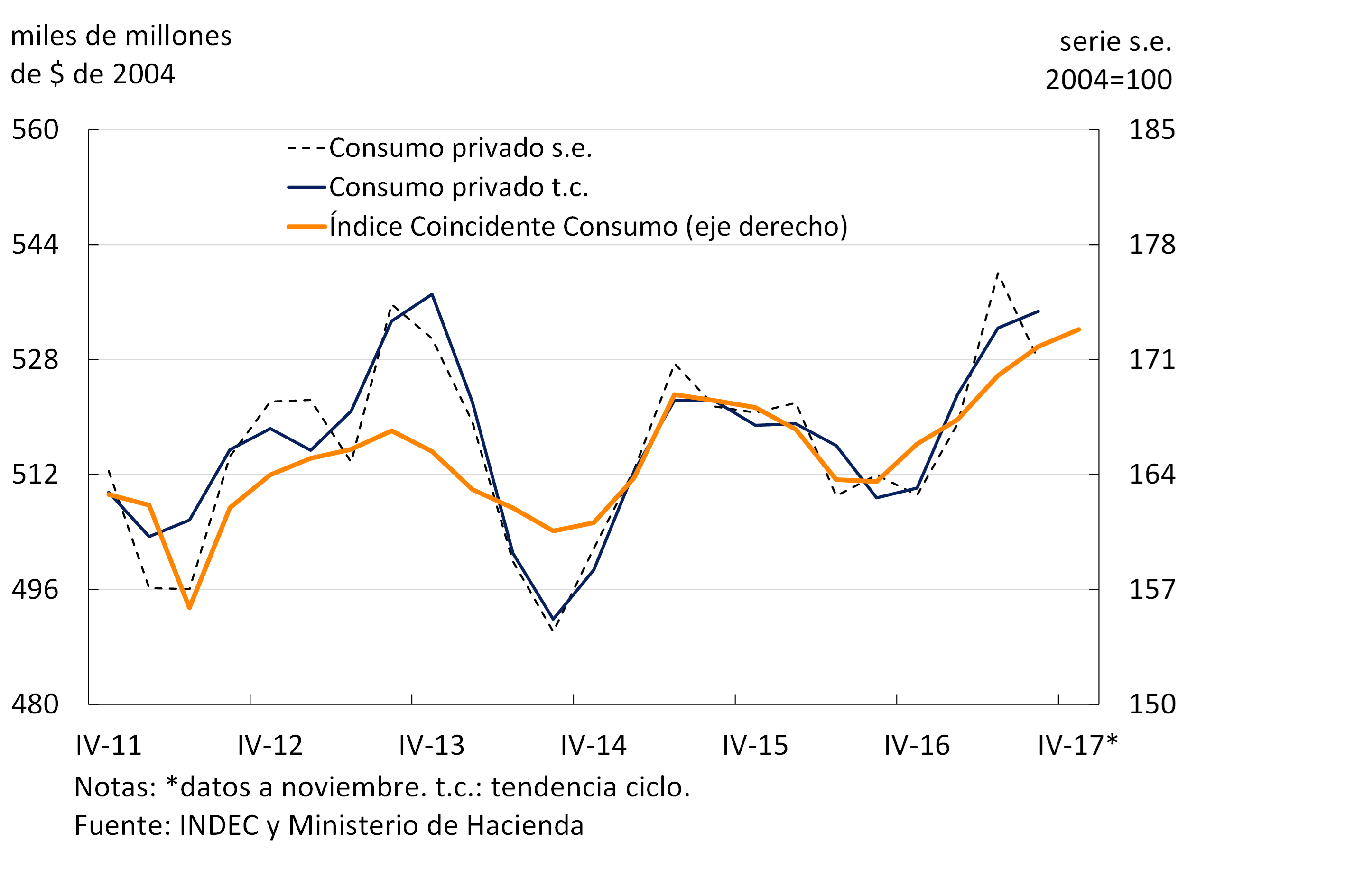
Private consumption increased 4.2% YoY in the third quarter of 2017 and fell 2.2% compared to the previous quarter in seasonally adjusted terms after an extraordinary 4% increase during the second quarter. Given the high volatility of the series beginning in 2004, it is appropriate to analyse the trend-cycle of consumption, which continued to grow during the third quarter (+0.4% s.e.)9.
Alternative indicators of private consumption indicate that it has grown uninterruptedly since the third quarter of 2016, in line with the trend-cycle of the official series. The BCRA’s Leading Indicator of Private Consumption—a monthly index that includes traditional indicators of consumption of goods and services, imports, consumer expectations, and indirect ways of calculating structural changes in consumption10—showed a turning point in October 2016, initiating an expansionary phase since then. The Coincident Consumption Index of the Ministry of Finance rose 0.6% s.e. in the fourth quarter after growing 1% s.e. in the previous quarter (see Figure 3.11).
Figure 3.11 | Evolution of private consumption
3.1.4 The negative current account is evidence of the expansion of domestic demand
The observed increase in the current account deficit in 2017 reflected the greater dynamism of local demand in relation to output. This evolution of the external accounts is to be expected after the macroeconomic reconfiguration that began at the end of 2015 and the new growth prospects. These, together with the reduction in the cost of using capital, have stimulated investment. To the extent that agents perceive an improvement in their permanent income and that they have access to credit, consumption is also expected to grow. Thus, the greater dynamism of investment vis-à-vis consumption leads to an increase in the current account deficit.
The greatest access to foreign savings is given from a very favorable stock position for our country, both at the aggregate level and by sectors. Argentina has an international investment position of approximately 5% of GDP, which makes it a net creditor of the rest of the world. Household and firm debt levels are very low, while the public debt-to-GDP ratio is below the average for countries in the region11.
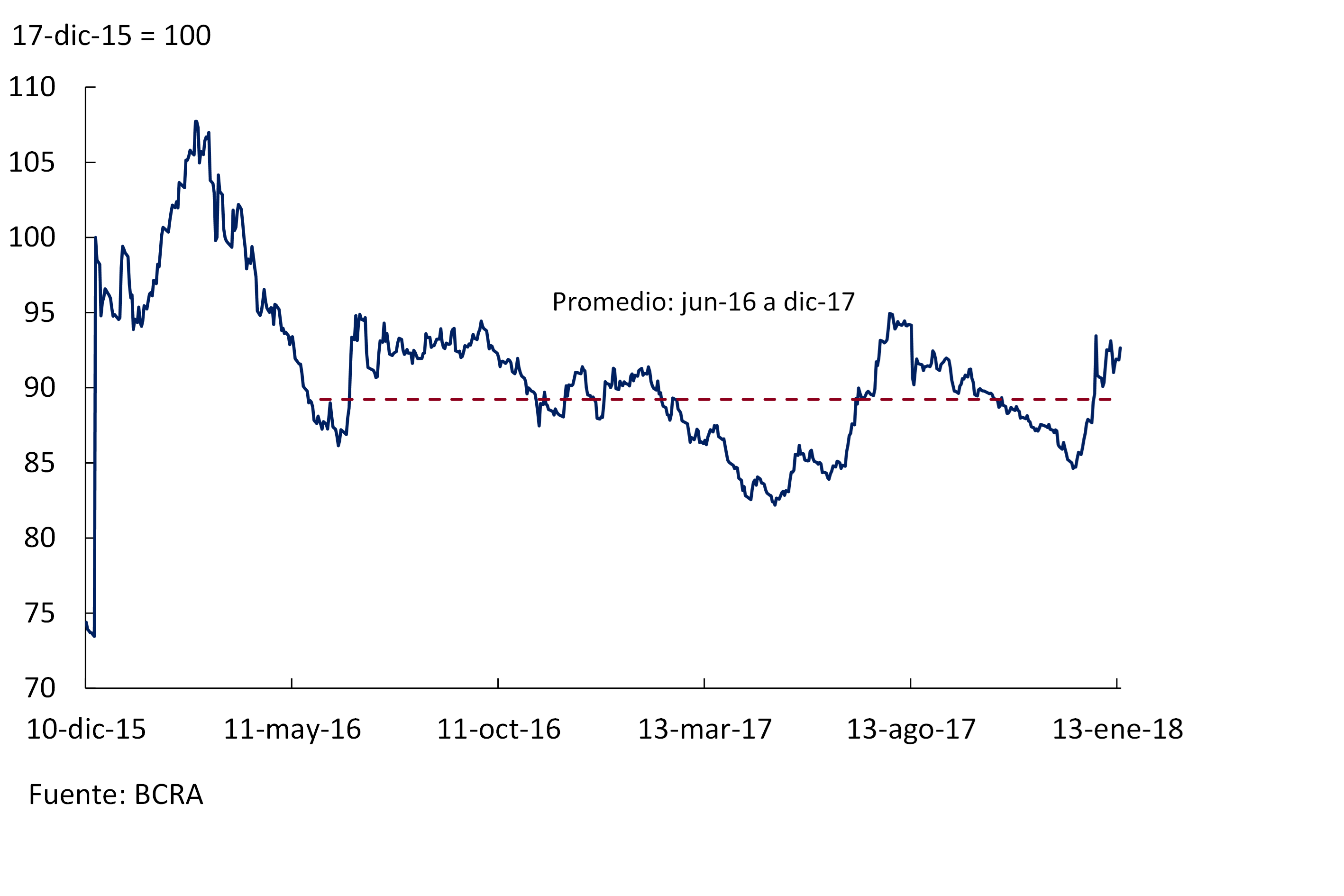
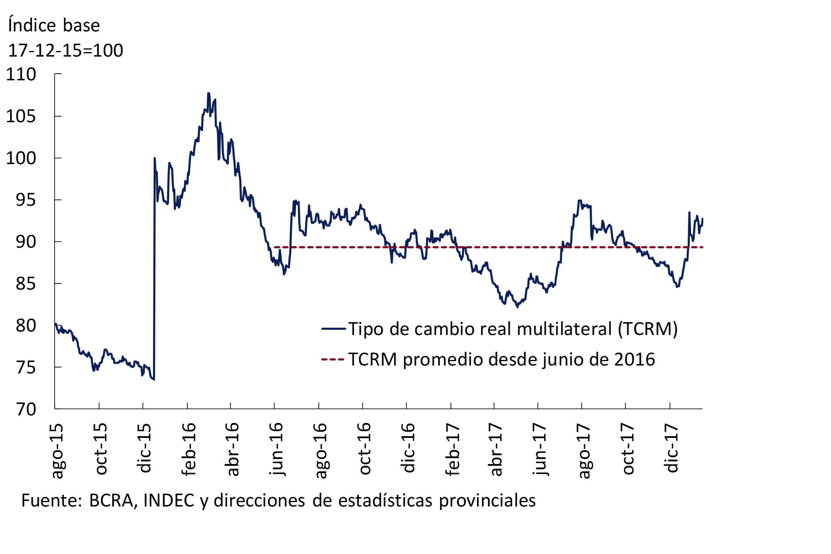
It should be noted that the increase in the current account deficit occurs in a context of relative stability of the multilateral real exchange rate (see Figure 3.12). In fact, as of December 31, 2017, the Multilateral Real Exchange Rate Index (ITCRM) was 0.5% above the value recorded exactly one year ago and 1.6% above the average since June 2016 (see Figure 3.12). In multilateral terms, the peso ended the year 23.4% more competitive than before the exchange rate unification of December 2015, as a result of a more marked depreciation with the Brazilian real (41.8%) than with the dollar (13.6%).
Figure 3.12 | Multilateral Real Exchange Rate
The larger current account deficit during 2017 was largely explained by the strong dynamism of imports of goods in a context in which exports remained practically stable. With data as of November 2017, export values accumulated an increase of 1.2% YoY (with a 1.1% increase in prices and a stagnation in quantities), well below the 19.9% YoY increase in imports, due to an increase in quantities (13.2% YoY) and in prices (6.0% YoY). The trade balance was reversed, going from a surplus of US$ 1,935 million between January and November 2016 to a deficit of US$ 7,656 million a year later.
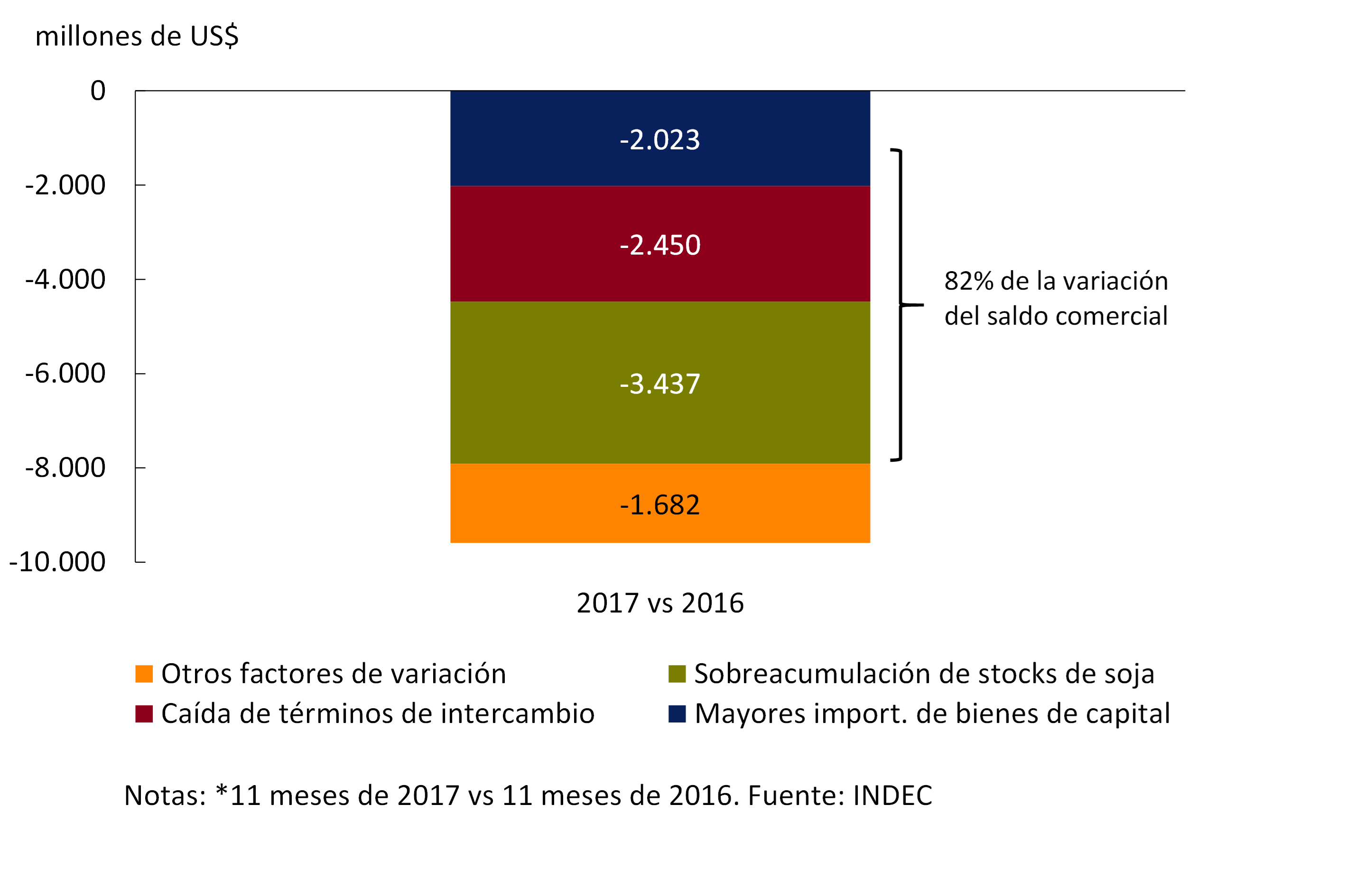
Box. Factors behind the increase in the trade deficit
More than two-thirds of the fall in the trade balance in 2017 was explained by the strong dynamism of foreign purchases linked to the investment process after years of stagnation, the deterioration of the terms of trade and the transitory accumulation of soybean stocks.
Figure 3.13 | Factors of change in the trade balance of goods*
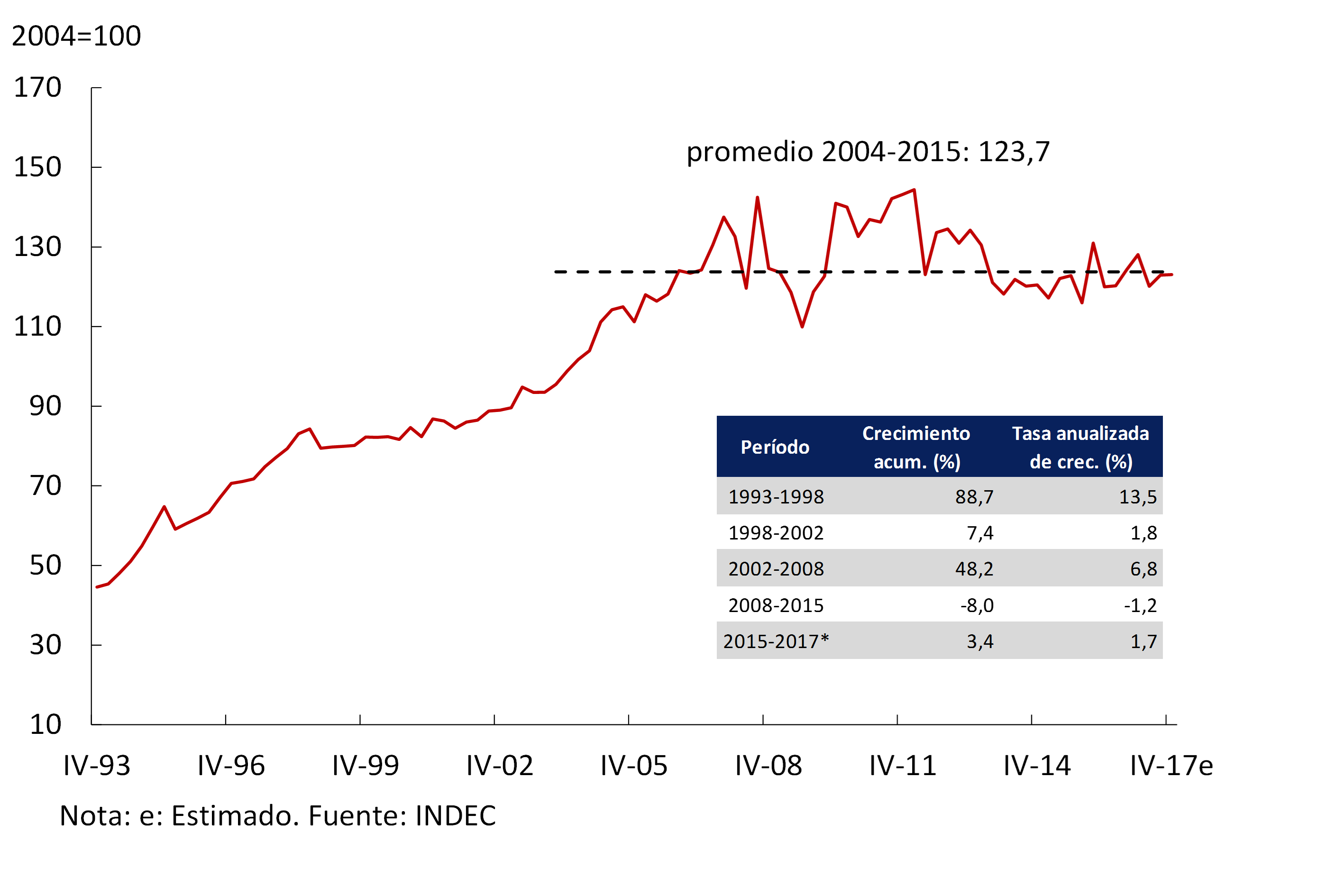
Exports have grown over the past two years, reaching levels similar to those recorded in 2006-2007, but have not yet broken the trend of stagnation of 2004-2015 (see Figure 3.14). During the first eleven months of 2017, the growth in foreign sales of Manufactures of Industrial Origin (MOI; 10% YoY) was offset by the falls in exports of primary products (PP; 6.2% YoY) and Manufactures of Agricultural Origin (MOA; 2.3% YoY). In the face of a record agricultural harvest, the fall in exports of primary products was explained to a greater extent by the retention of soybean stocks by producers. In MOA exports, the behavior was heterogeneous with increases in meat (22% y.o.y.) and falls in dairy products (27% y.o.y.) and soybean by-products (3% y.o.y.).
Figure 3.14 | Exported quantities of goods and services
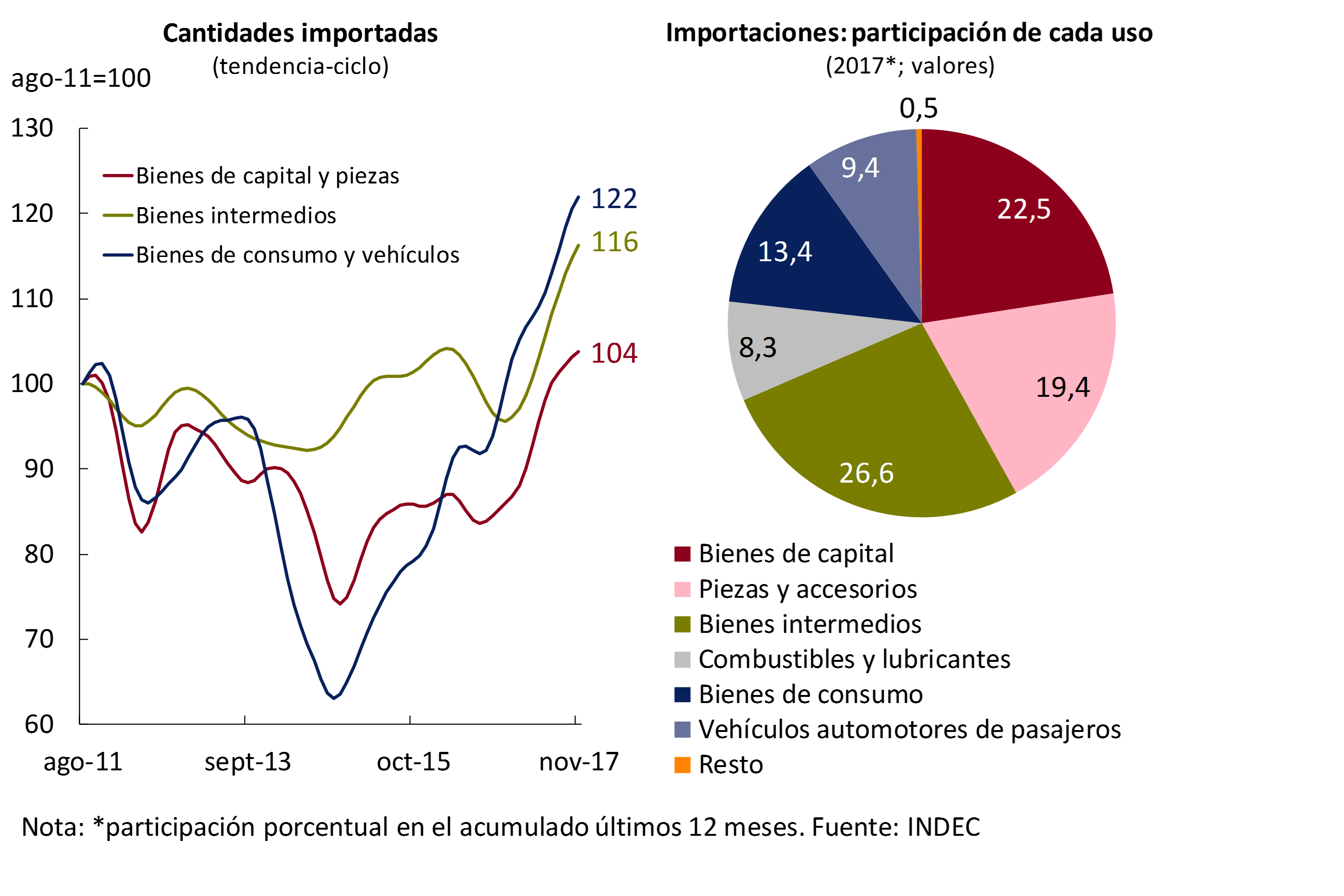
Imported quantities of goods continued to grow, reaching record levels in relation to the level of economic activity. The dynamism of foreign purchases of capital goods and their parts associated with the strong investment process that characterizes the current expansion phase was highlighted. Imports of consumer goods and automobiles also contributed, favored by the elimination of distortions in foreign trade of these products, but with a lower weight in the country’s imports as a whole (see Figure 3.15.).
Figure 3.15 | Evolution and composition of imports of goods
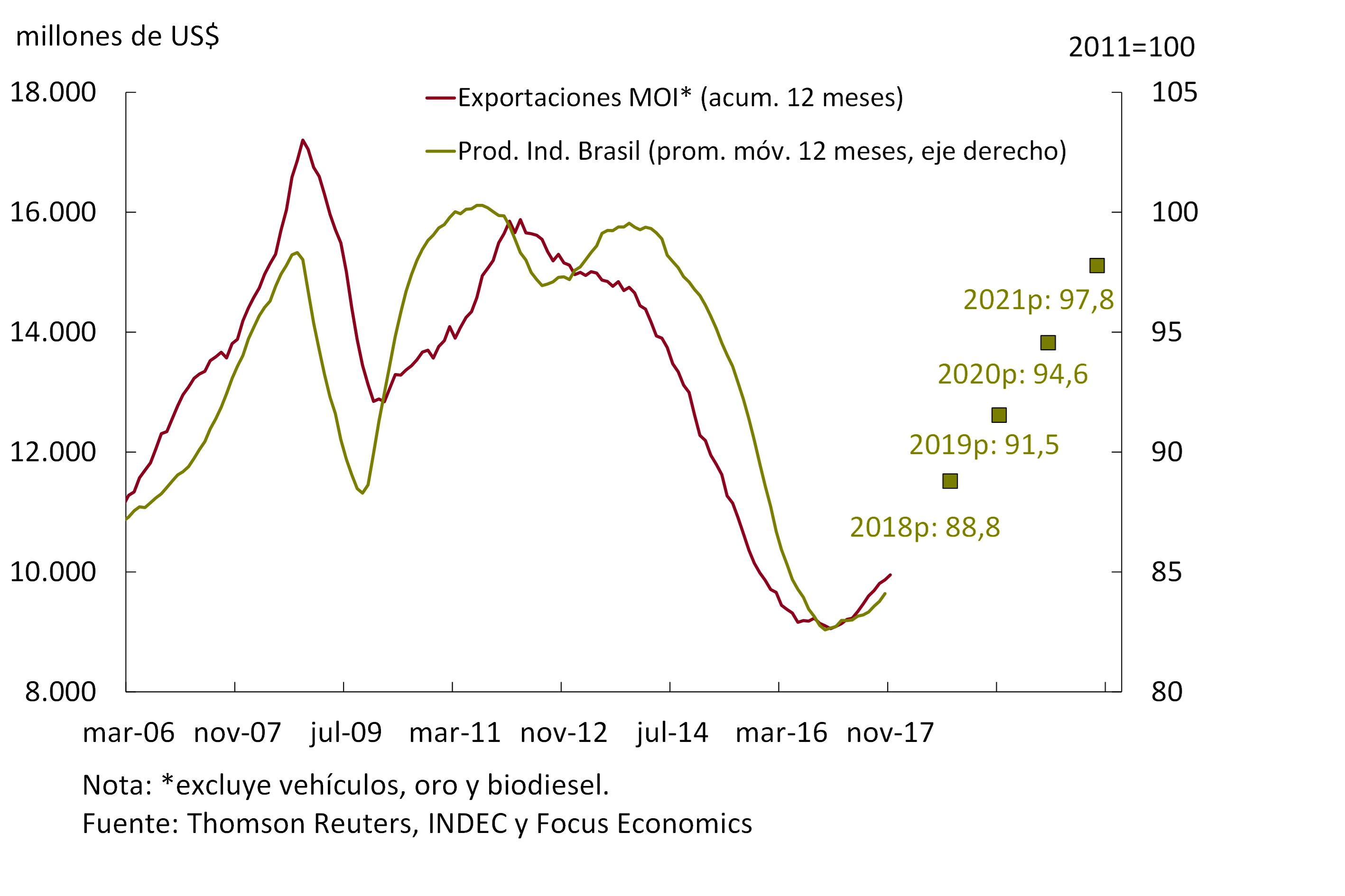
In the medium term, the external accounts are expected to continue to reflect the strong dynamism of domestic demand. Imports will continue to grow in all their uses, with emphasis on those associated with the investment and production process. The export items that have the most favorable prospects in the current situation are those that could benefit from the higher projected growth in the economic activity of our main trading partners. In particular, industrial manufacturing will be helped by the recovery of industrial activity in Argentina’s main trading partner, Brazil (see Figure 3.16).
Figure 3.16 | Brazil Selected Industrial Manufactures Exports and Industrial Production
3.1.5 Productivity increases and spreads across sectors
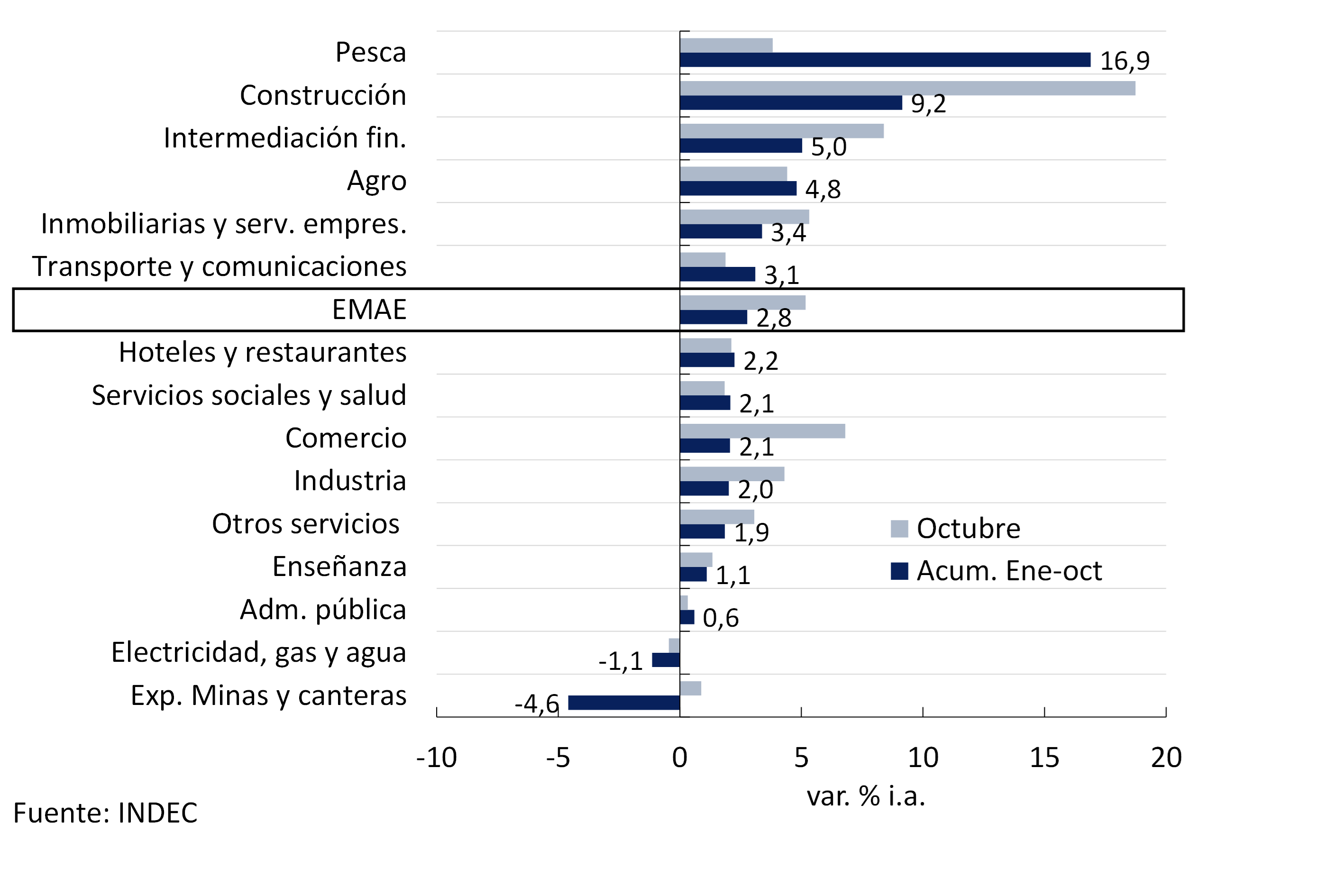
Economic growth was widespread among the productive sectors in the course of 2017. The average of the diffusion index, which counts the percentage of items that grew month by month, was around 59% between January and October.
Among the most dynamic activities in the last year are fishing, construction, financial intermediation, the agricultural sector and real estate services. Construction continues to be driven by private and public works. Financial intermediation was driven by the drop in expected inflation that allows the credit horizon to be extended, the implementation of measures aimed at facilitating the operation of the banking system12 and the strong demand for credit in UVAs, which is growing at a rate of more than 90% per year. Agricultural production continues to respond positively to the elimination/reduction of export duties and trade and exchange rate normalization beyond the high retention of stocks that impacts grain exports.
The only sectors that contracted in the January-October 2017 average compared to the same period of the previous year were electricity, gas and water (EGA), and mining and quarrying. In the first case, the sector was affected by the fall in residential demand due to higher temperatures compared to the previous year and the reduction of subsidies. In the second, international oil prices prevailing in the period were not profitable to break the declining trend in production that has been evident since 1998, while mining activity fell as a result of the reduction in exploration work in previous years (see Figure 3.17).
Figure 3.17 | Economic growth by productive sector
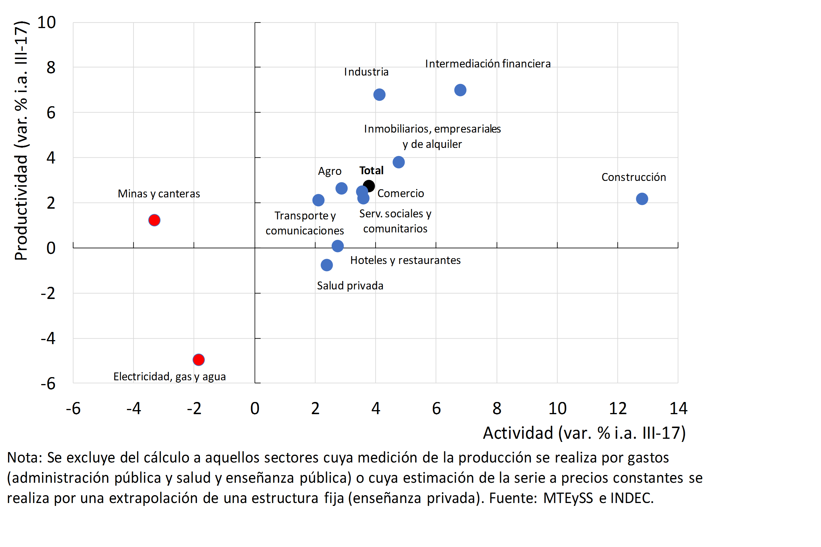
Growth was supported by an improvement in productivity per registered worker (2.7% YoY), consistent with the greater role of investment. Productivity gains were disseminated at the sectoral level (see Figure 3.18).
Figure 3.18 | GDP and productivity (sectoral GDP/employment registered in the sector)
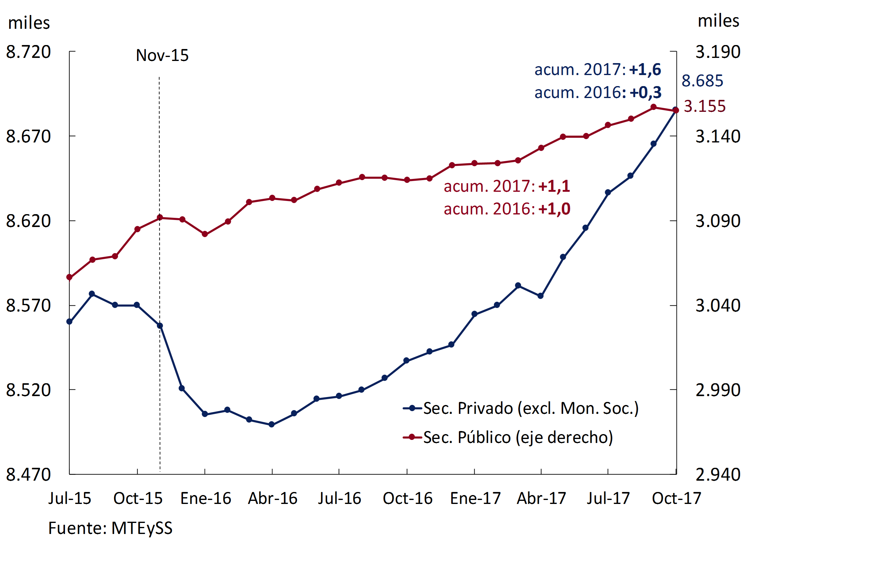
In the year, sectoral employment continued to be led by construction (8.5% YoY), electricity, gas and water (2.7% YoY) and fishing (1.6% YoY), while among services the most dynamic sectors were hotels and restaurants (2% YoY) and community, social and personal services (1.5% YoY). It was followed by moderate growth in real estate, business and rental services (1.1% YoY), and Trade and Repairs (1.0% YoY). Since April 2017, job creation has accelerated, driven by greater dynamism in the private sector, which accounted for 81% of the creation of new registered jobs (see Figure 3.19)13.
Figure 3.19 | Registered workers in the public and private sectors
Unemployment and underemployment rates did not register significant variations between the third quarters of 2016 and 2017, as the labor supply and the employment rate increased in a similar way (0.3 p.p.).
At the end of the third quarter of 2017, there was a slight improvement in the distribution of per capita income14, driven by the slowdown in inflation and measures aimed at improving the disposable income of the most vulnerable sectors, such as the VAT refund for retirees and pensioners and AUH beneficiaries. This improvement occurred within the framework of a recovery in real wages. In particular, the remuneration of registered private wage earners rose in real terms by 5.3% YoY in the July-September 2017 average15.
3.2 Growth prospects for the next two years consolidate
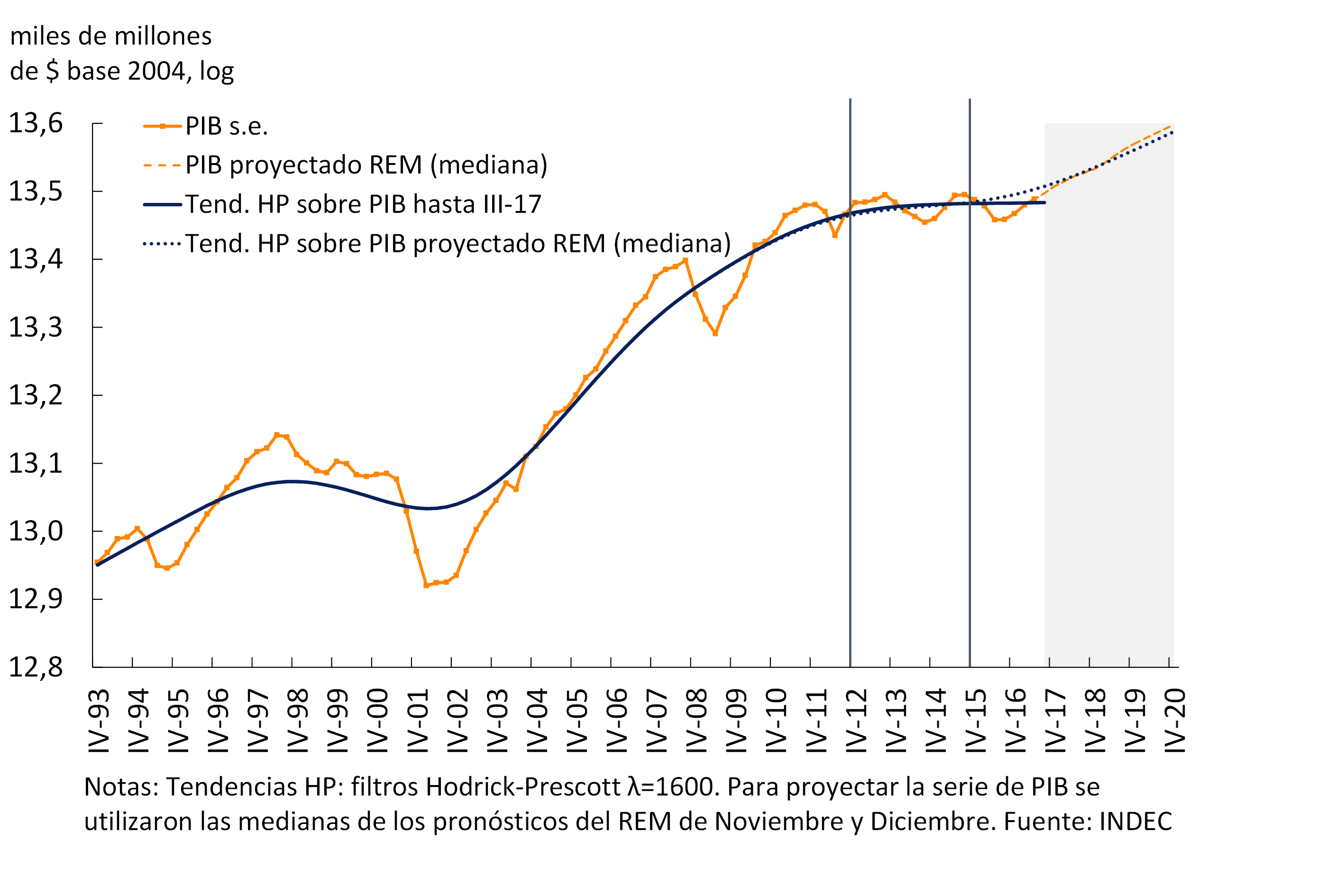
The economy completed a year of uninterrupted growth at an annualized rate of 4% during 2017. The BCRA expects sustained growth to continue, while becoming less volatile, leaving behind the stage of trend stagnation of output. This view is in line with the estimates included in the 2018 National Budget Law, which contemplates a growth of 3.5% for 2018-2019 and is shared by the participants of the Market Expectations Survey (REM) who projected that the economy will continue to expand annually by 3.2%, 3.3% and 3.2% in 2018, 2019 and 2020 respectively. The increases in GDP expected by analysts for the coming years imply a break in the economy’s long-term growth trend (see Figure 3.20).
At the end of 2015, a series of measures were adopted to correct the macroeconomic imbalances that allowed the growth path to be recovered, with increases in employment, productivity and a leading role for investment. The recently passed tax reform law and the agreements with the provinces aim to reduce those taxes that affect the competitiveness of the economy, particularly distortionary ones, and to increase the rate of return on capital16. These structural reforms are important to boost Argentina’s economic potential in a sustained manner (see Section 1 / Impact of structural reforms on productive sectors).
The Government announced fiscal targets that imply a reduction in the primary deficit of the national non-financial public sector from 3.9% of GDP (which was 0.3 percentage points lower than the target set for 2017) to 3.2% in 2018, 2.2% of GDP in 2019 and 1.2% of GDP in 2020. A gradual reduction in the tax burden is expected from the recent enactment of the tax reform law and the gradual reductions planned for export duties on the soybean complex. Domestic primary expenditure will fall by around 1 percentage point of GDP in 2018, while the gradual reduction of subsidies, mainly in energy and transport, is expected to continue. On the other hand, spending on social assistance will increase in real terms during 2018. Investment in infrastructure will continue to increase, supported by the initiatives within the framework of public-private partnerships promoted by the Government.
The use of productive factors is below the level that would cause inflationary pressures, a dynamic that will continue to be monitored by the BCRA. It is estimated that in 2017 the GDP gap narrowed to -1.6%, from a value of -2.8% in 2016 (see Section 2 / The output gap: A small multivariate model). This decline is the result of growth of around 1.6% in potential GDP, defined as that which prevails in the absence of both inflationary and deflationary pressures, which was lower than what GDP is estimated to have experienced in 2017. Consequently, there is a trend towards the closing of the GDP gap, although without signs of inflationary pressures.
Figure 3.20 | GDP trend based on REM projections
4. Pricing
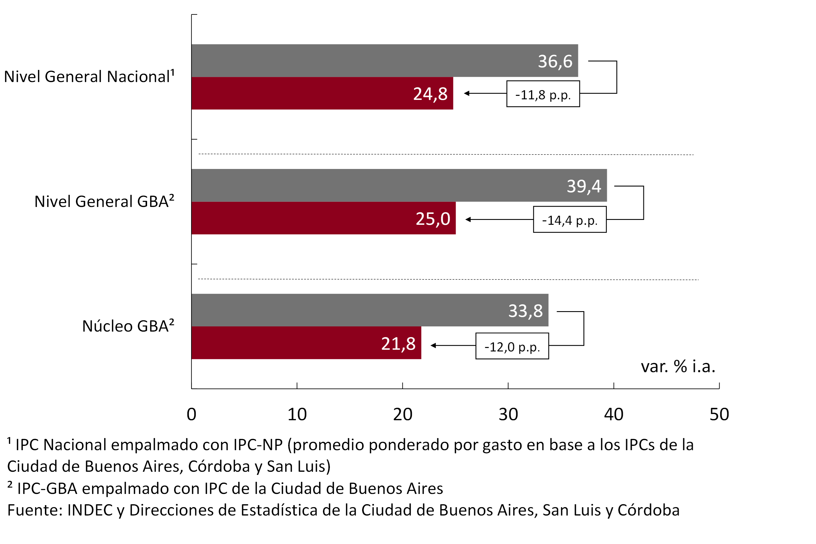
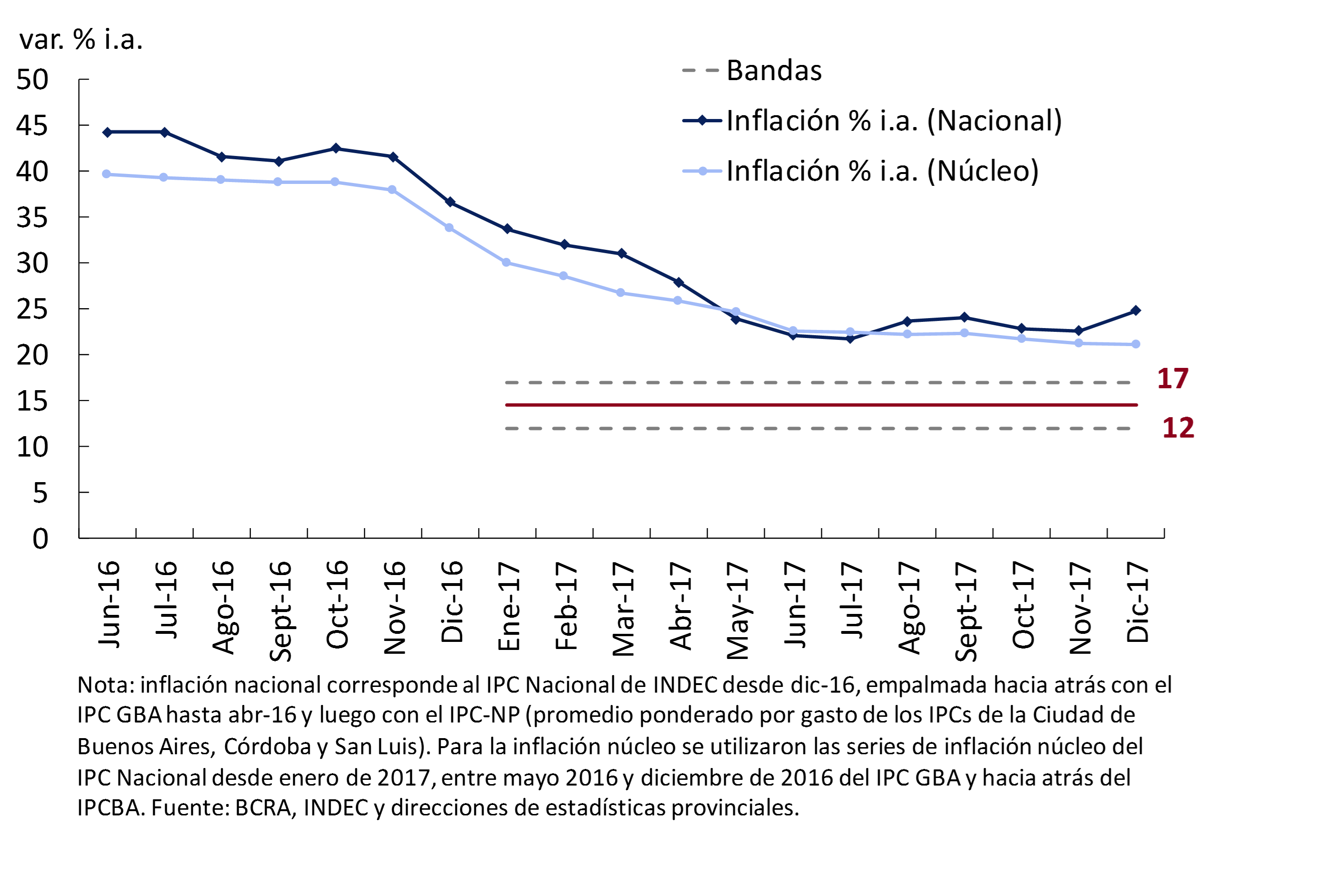
The year 2017 ended with inflation of 24.8% YoY, marking a drop of 11.8 percentage points compared to the previous year17. This slowdown occurred in a context of free floating of the exchange rate and the recomposition of public service rates. Core inflation stood at 21.1% YoY, the lowest variation since 2009.
Core inflation, on which monetary policy operates, continued to decelerate during the latter part of the year. This dynamic was observed beyond the direct impact that the increases in the rates of public services concentrated in December had on it. The increase in the core component was 1.4% monthly average in the last quarter of 2017, the lowest in the last six years.
Market analysts’ inflation expectations expect disinflation to continue in the coming years. The estimates for 2018 were revised slightly upwards compared to the previous IPOM, basically responding to an upward correction in regulated prices.
4.1 Inflation slowed during 2017
Inflation slowed significantly during 2017, with a fall of 11.8 percentage points (p.p.) compared to the previous year, according to the national indicator, and 14.4 p.p., according to the GBA18 CPI. In December, core inflation stood at 21.1% YoY, 12.7 p.p. below 2016, the lowest since 2009. The prices of regulated goods and services (38.7% YoY) adjusted above the general level, while Seasonal prices (21.5%) increased in line with core inflation (see Figure 4.1).
Figure 4.1 | Year-on-year inflation. General Level and Core
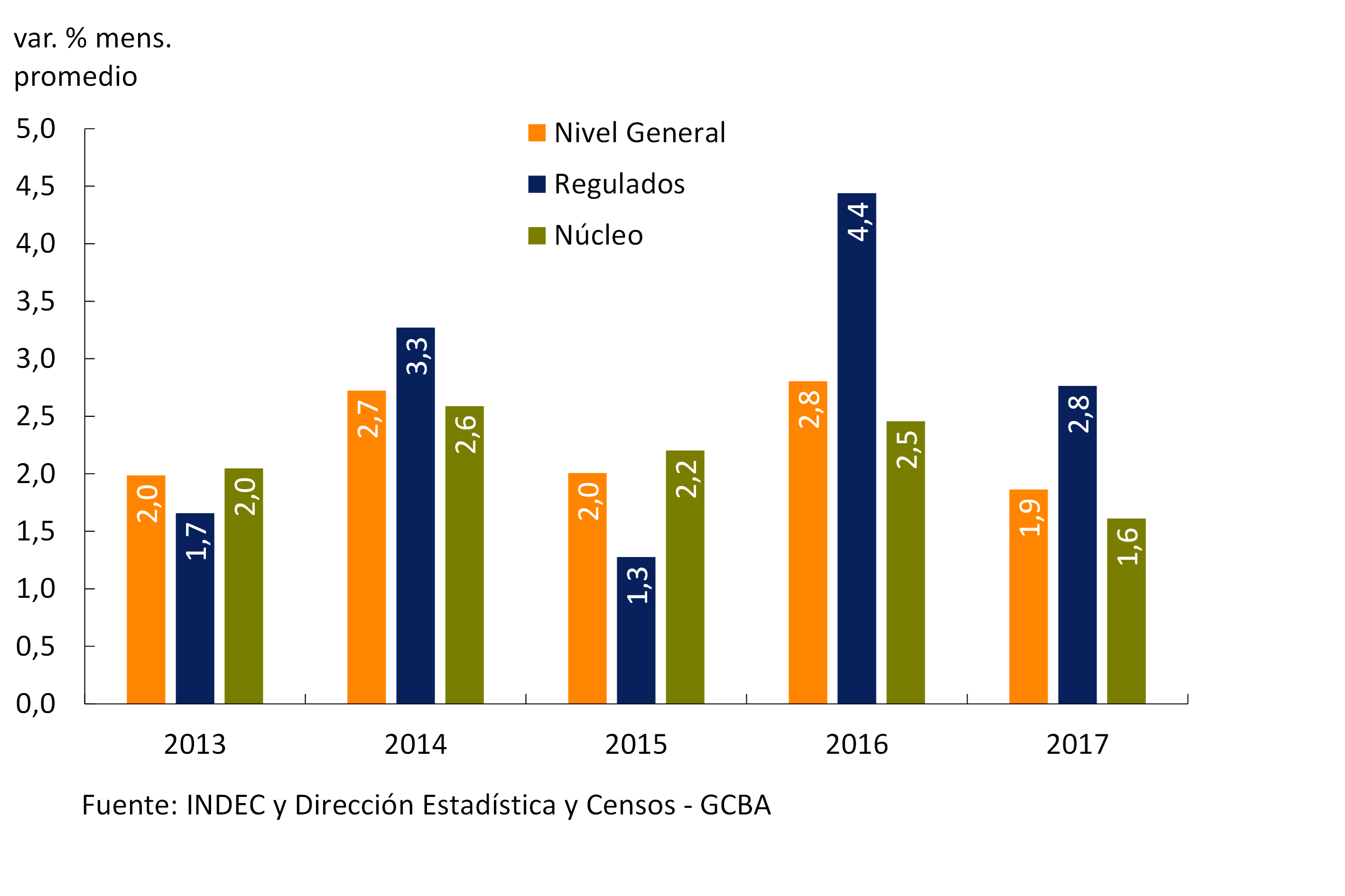
The disinflation achieved in 2017 was due to a sharp slowdown in core inflation, in a context of recomposition of the relative prices of regulated services. In 2017, the average monthly rate of increase in core inflation was 1.6%, the lowest in recent years; meanwhile, the average growth of Regulated Entities was 2.8%. The latter accounted for more than 30% of inflation, a higher proportion than in other recent years with similar inflation (2013 and 2015; see Figure 4.2).
Figure 4.2 | Inflation. Average Rates of Increase by Component
In the last quarter, the average monthly variation of the CPI increased as a result of the adjustments of Regulated items, driving an acceleration in year-on-year terms. Specifically, in December there were increases in the rates of public services (electricity and gas), gasoline and prepaid. In the last month of the year, the Regulated Index registered a monthly variation of 9.1%, leading inflation to grow at a rate of 3.1%.
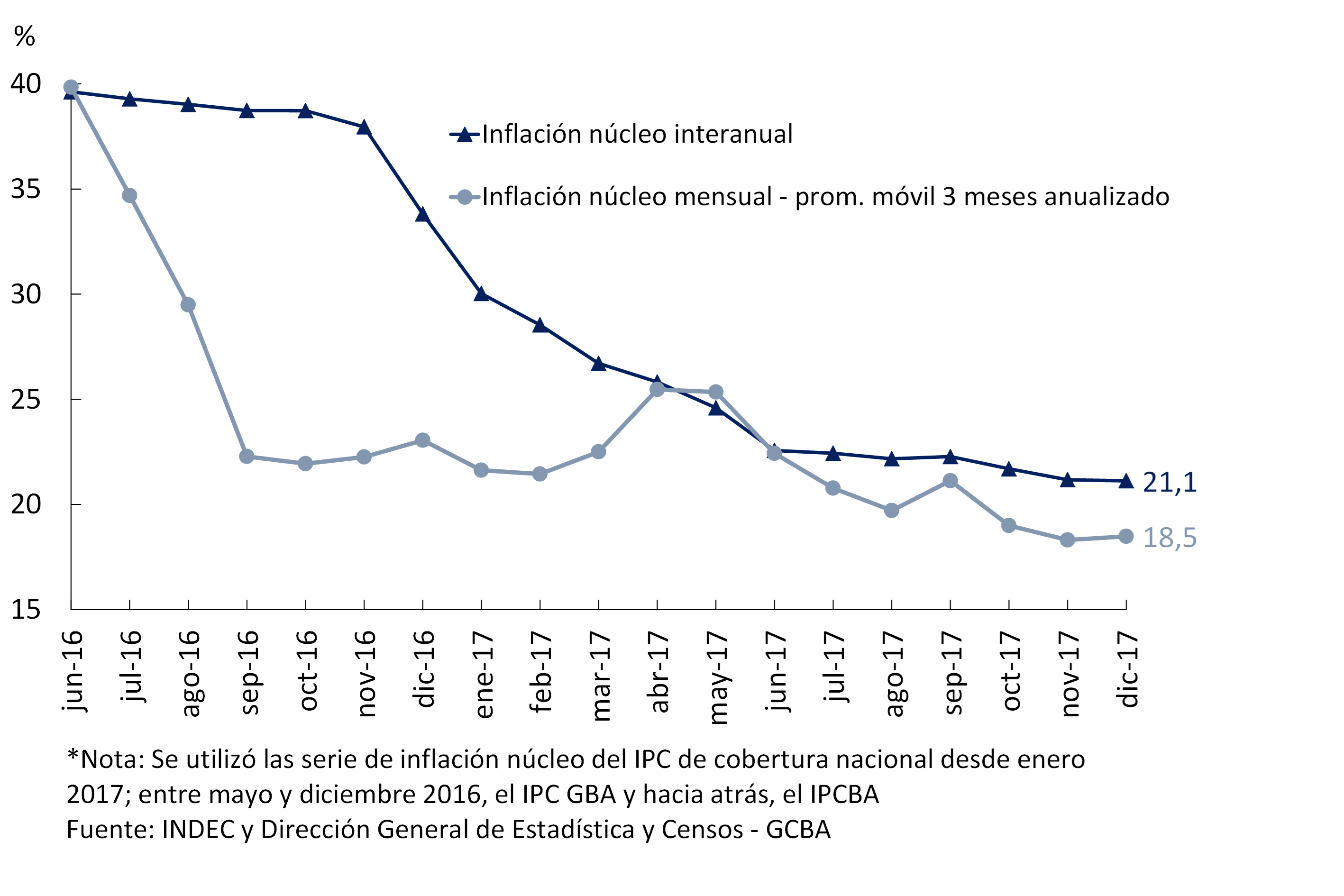
During the fourth quarter, core inflation continued to decelerate despite the direct impact of the rise in energy inputs (electricity and gas) on expenses19. Some one-off salary increases such as those for domestic service and building managers also pushed up core inflation through an annual bonus. The three-month moving average of monthly core inflation registered the lowest in the last six years, standing at 18.5% in annualized terms (see Figure 4.3).
Figure 4.3 | Core inflation. CPI
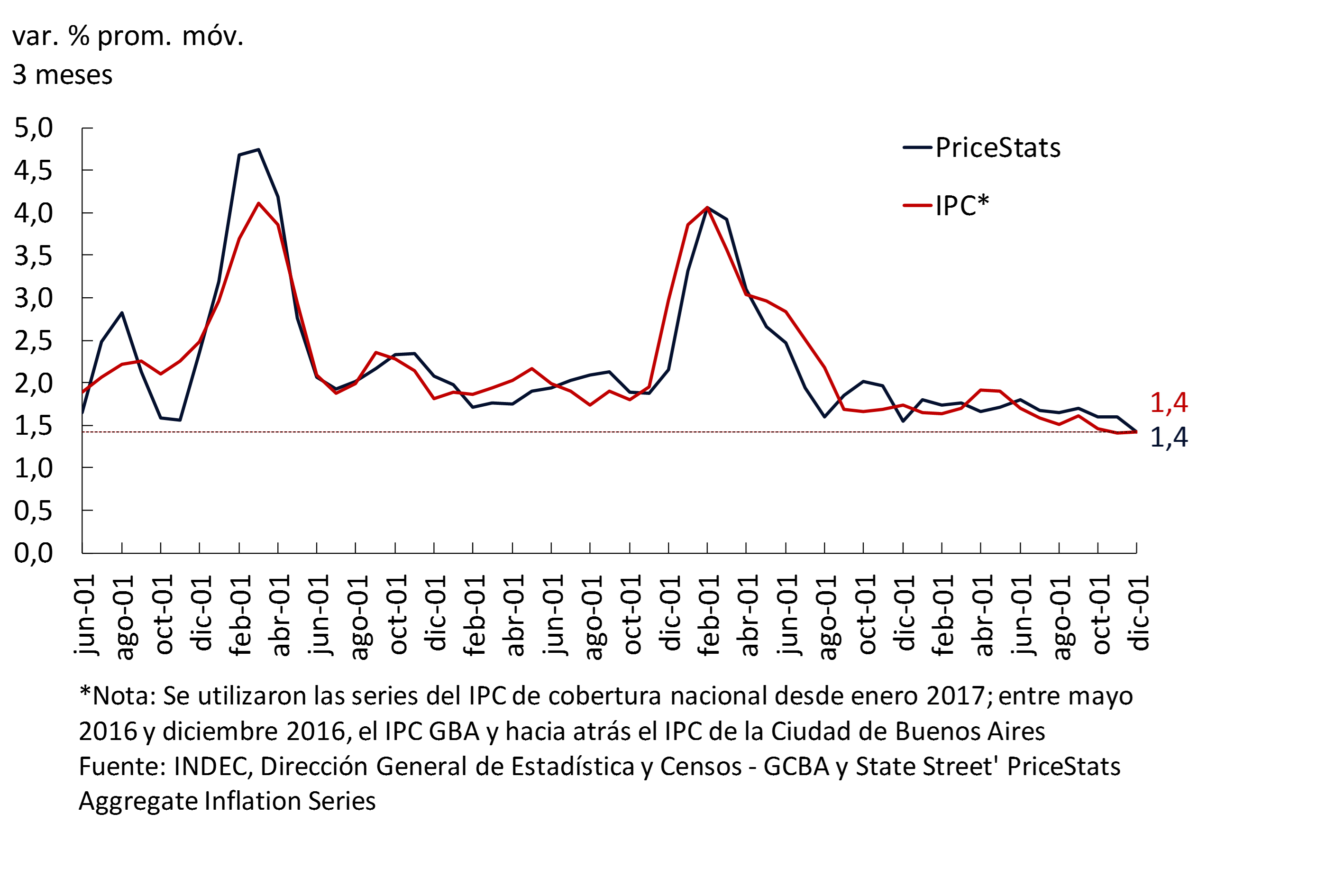
Various high-frequency indicators available, which have a high correlation with the evolution of core inflation, also showed a slowdown in the last months of the year. The index prepared by PriceStats grew at a monthly rate of 1.4% in the last quarter of 2017, after having exhibited a rate of increase of 1.7% in the first part of the year (see Figure 4.4).
Figure 4.4 | Core inflation and leading indicators
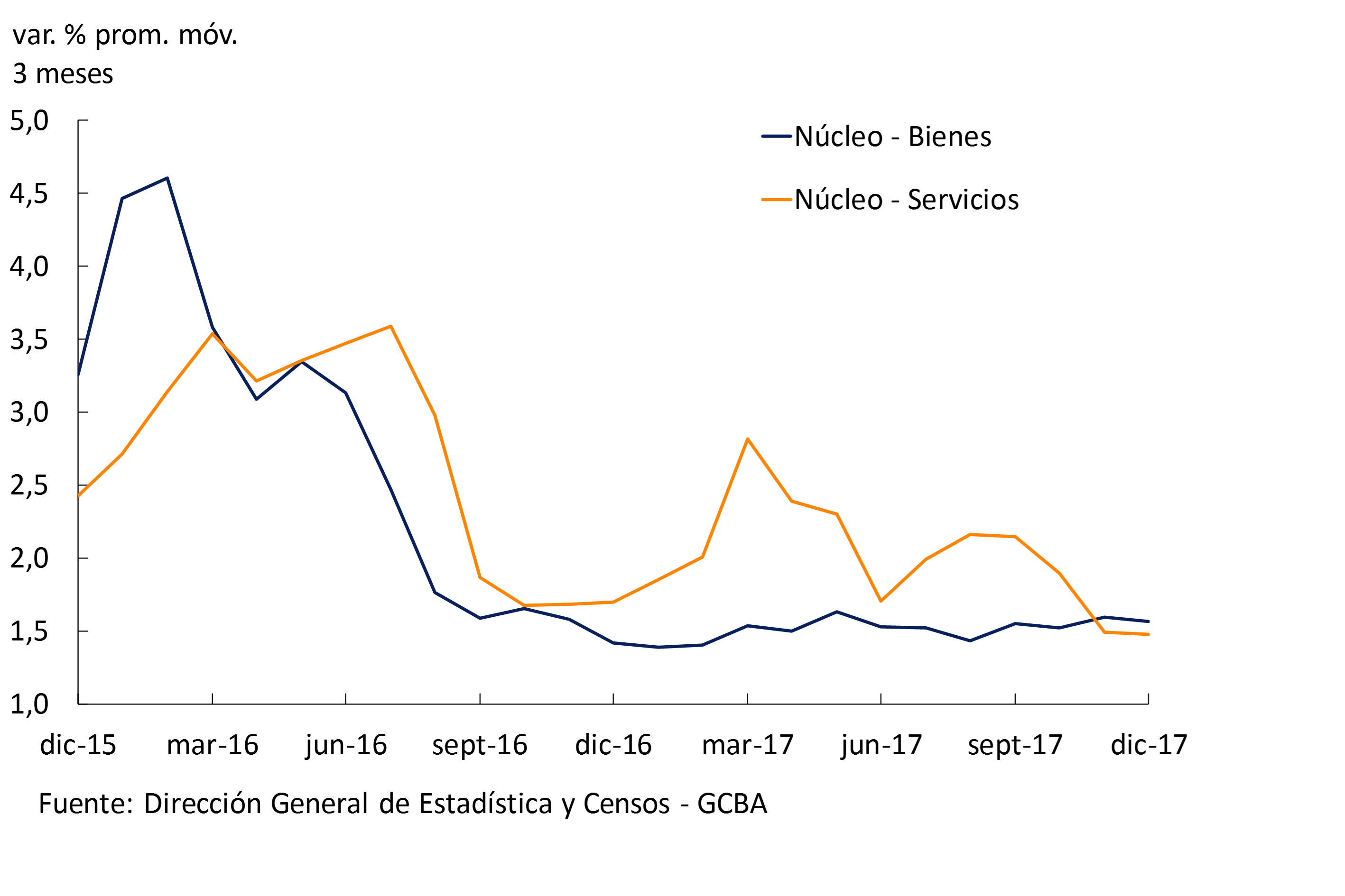
The breakdown of core inflation into goods and services20 shows a slowdown in services in the fourth quarter of the year. This dynamic is consistent with the evolution of wages. Goods maintained a relatively stable and limited rate of growth during the year, with a behavior decoupled from fluctuations in the nominal exchange rate. The relationship between the prices of private goods and services remained relatively stable in the last quarter (see Figure 4.5).
Figure 4.5 | CPI CABA. Core inflation decomposition
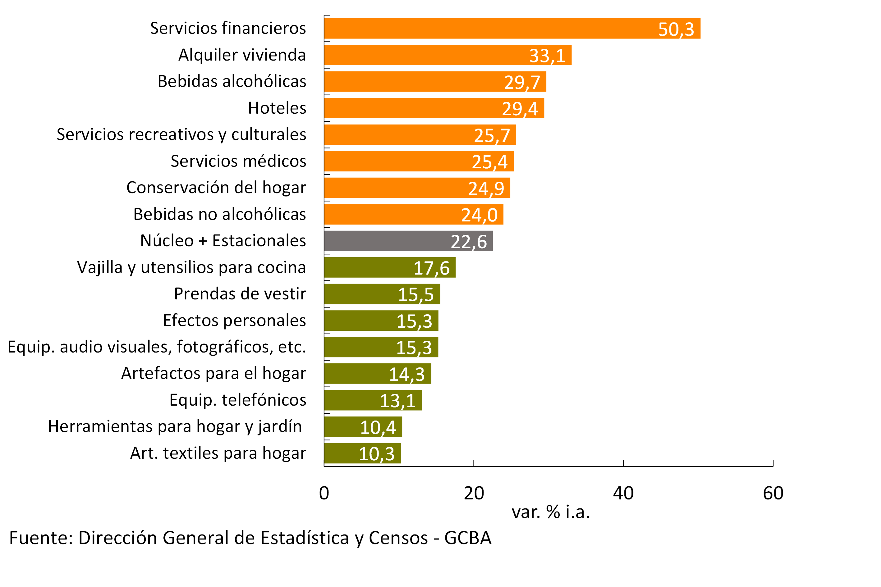
Goods prices contributed mostly to the year-on-year slowdown in core inflation, resulting in a relative decline in the prices of goods relative to private services. As of December 2017, 25% of the groups that increased the most in year-on-year terms corresponded mainly to services, among which rentals, financial services, tourist accommodation and recreational services stood out. At the other extreme, the smallest price increases correspond basically to groups with a high component of goods, which are more exposed to external competition and technological progress (see Figure 4.6). Specifically, food for consumption at home, which represents approximately 18.6% of the core component plus seasons, registered a year-on-year increase of 20.5%, slightly lower than the average for the aggregate.
Figure 4.6 | CPI CABA 2017 by groups. First and fourth quartile
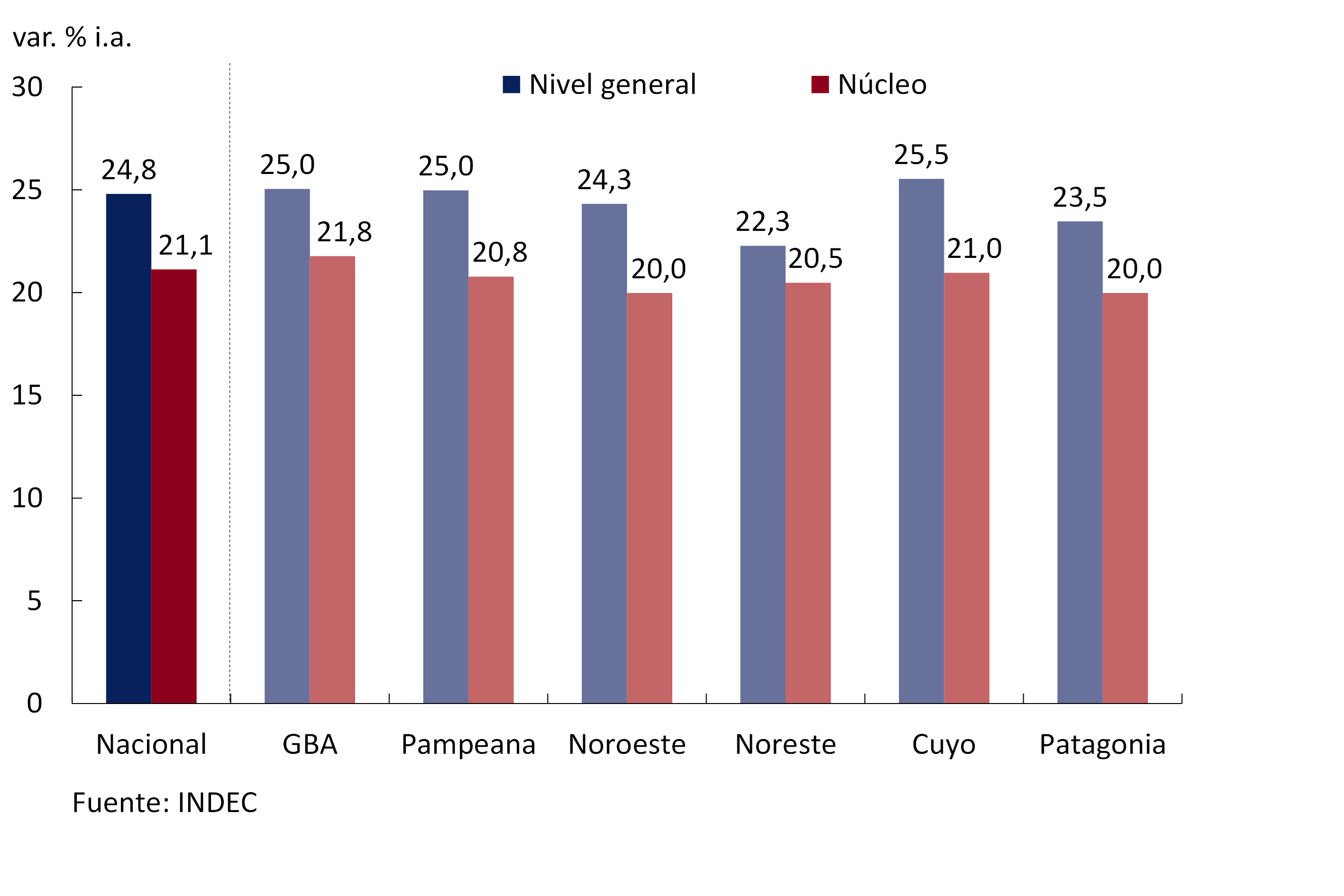
At the regional level, core inflation was relatively homogeneous in 2017. However, some differences in the evolution of regulated goods led to general inflation being slightly more heterogeneous. The Northeast accumulated the lowest increase in the general price level in year-on-year terms, growing 22.3%, while Cuyo exhibited the largest increase (see Figure 4.7).
Figure 4.7 | Year-on-year inflation by region
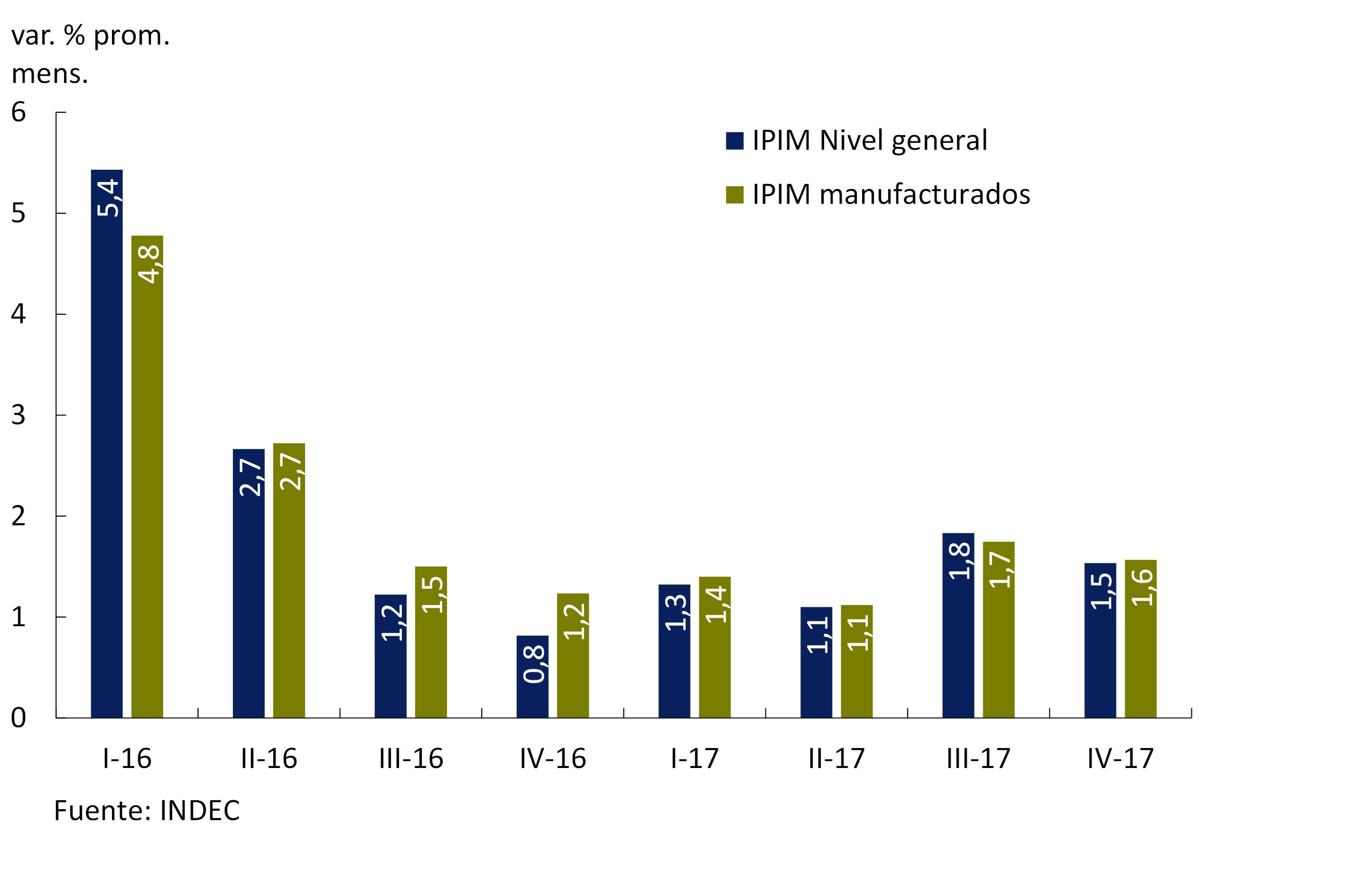
Wholesale prices21 ended 2017 with an increase of 18.8% YoY, 15.7 p.p. below 2016. These prices, mostly tradable, grew at rates similar to those of goods in the national CPI and ended the year with a year-on-year increase that was 6 p.p. below consumer prices (National CPI). The average variation of the last quarter was 1.5%, slowing down 0.3 p.p. compared to the previous quarter. The lowest rates of increase were recorded in most of its components (see Figure 4.8).
Figure 4.8 | IPIM. General and Manufactured Level
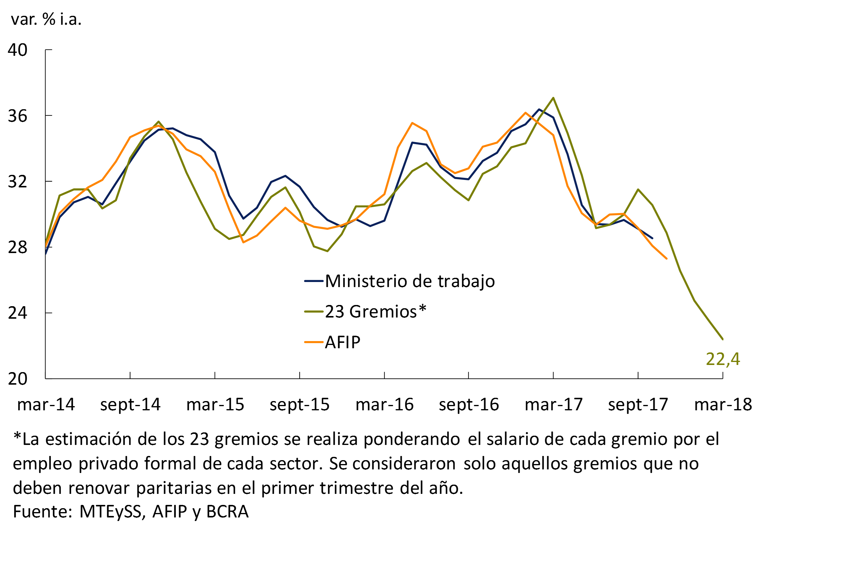
4.2 Nominal wages moderated their growth rate
In the fourth quarter, nominal wages would have increased at a lower rate than in the previous quarter. This dynamic was due to the fact that the structuring of the parity agreements practically did not contemplate adjustments for the last months of the year.
Most of the clauses for adjustment or revision of the salary guideline included in the collective bargaining agreements did not come into force, given that inflation was below the agreed wage increases. The nominal wage would have ended 2017 with an increase 2% higher than that of the accumulated inflation in the same year. At the beginning of 2018, the pace of year-on-year increase in wages would continue to slow (see Figure 4.9).
Figure 4.9 | Nominal wages. Formal private sector
It is estimated that the wage negotiations in 2018 will maintain the modality applied during 2017, in which the future dynamics of prices became relevant to the detriment of past developments. In this framework, wage negotiations are expected to be consistent with inflation targets for the year. Likewise, clauses could be contemplated that allow adjustments if inflation exceeds a certain threshold.
4.3 The path of disinflation would continue in 2018
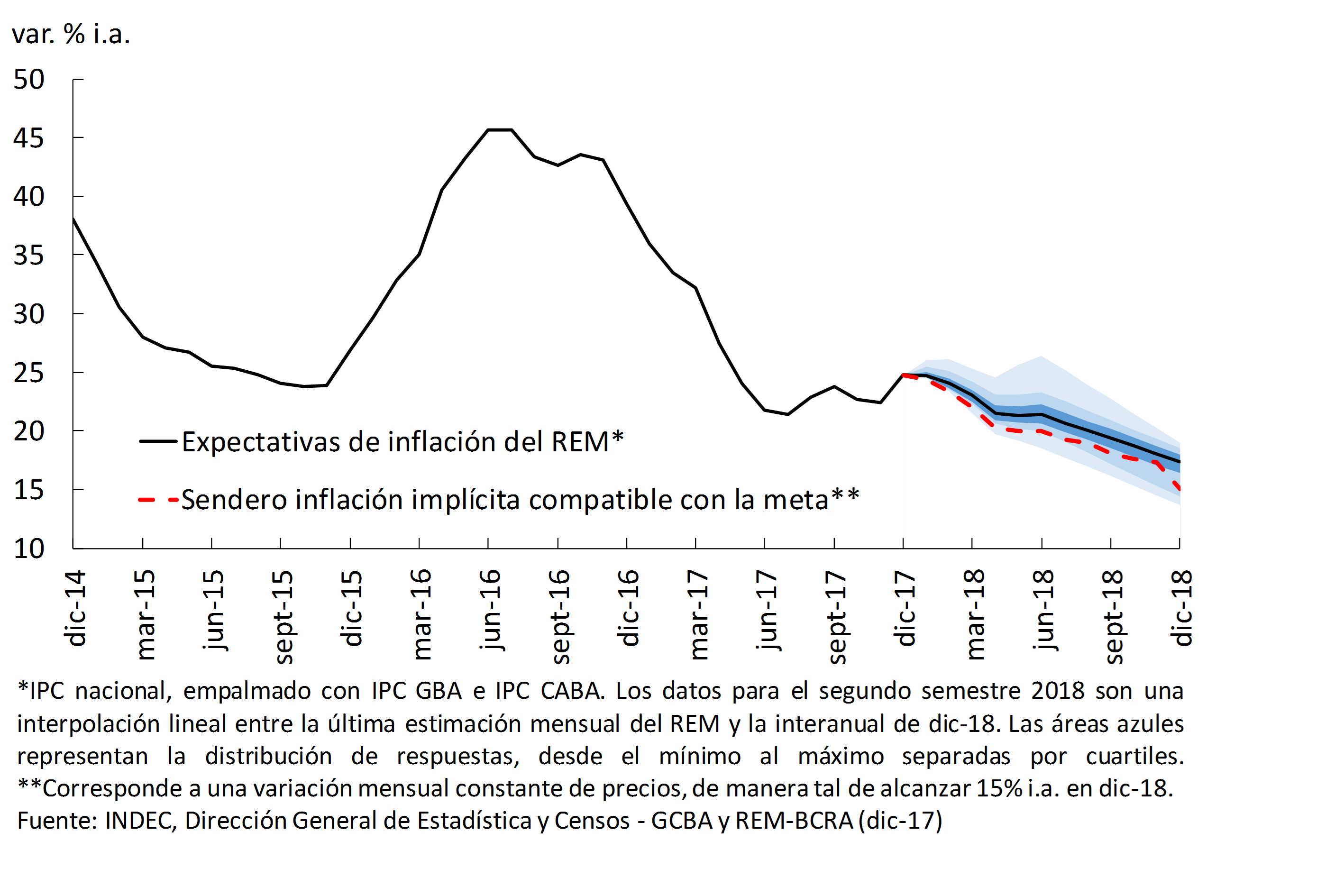
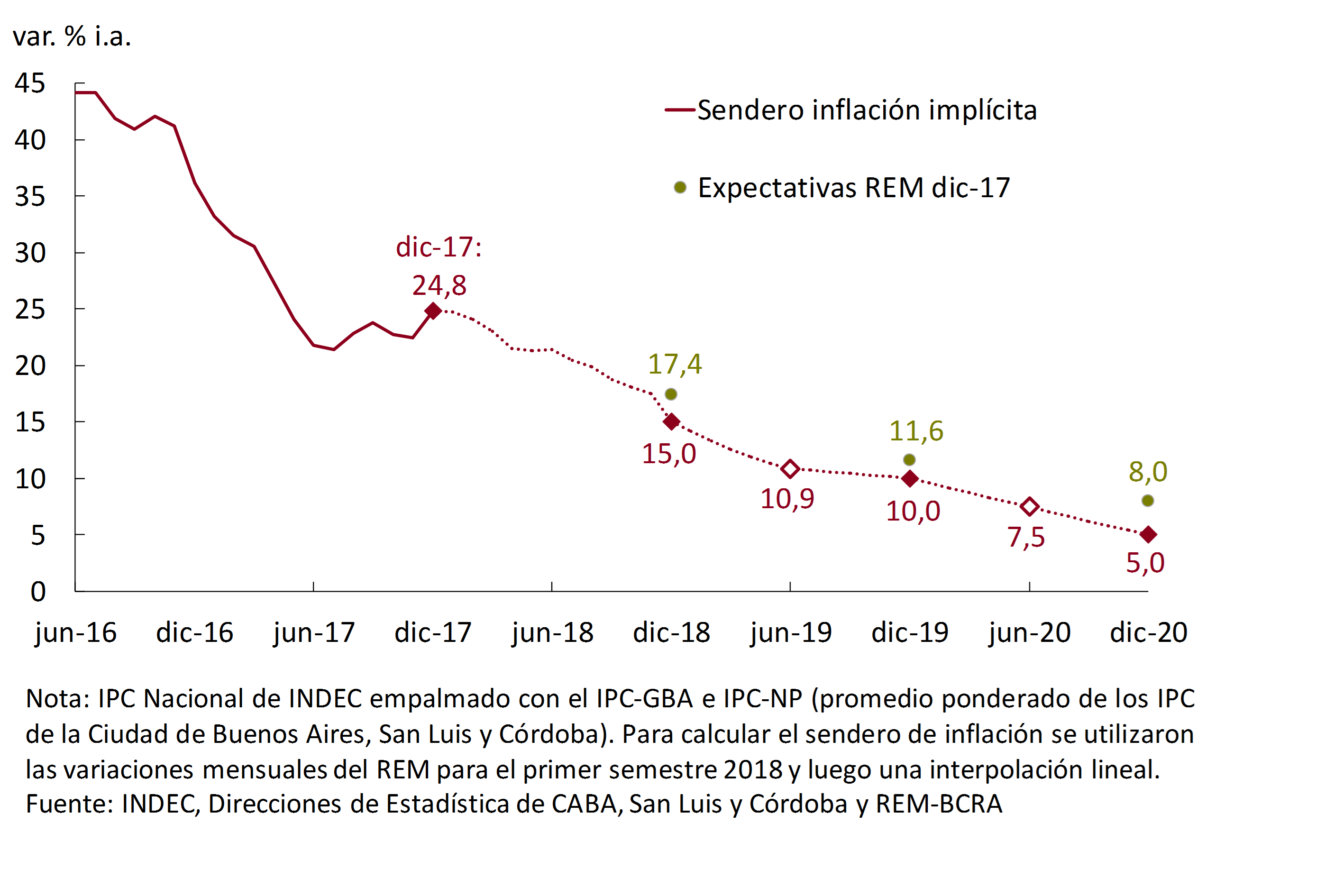
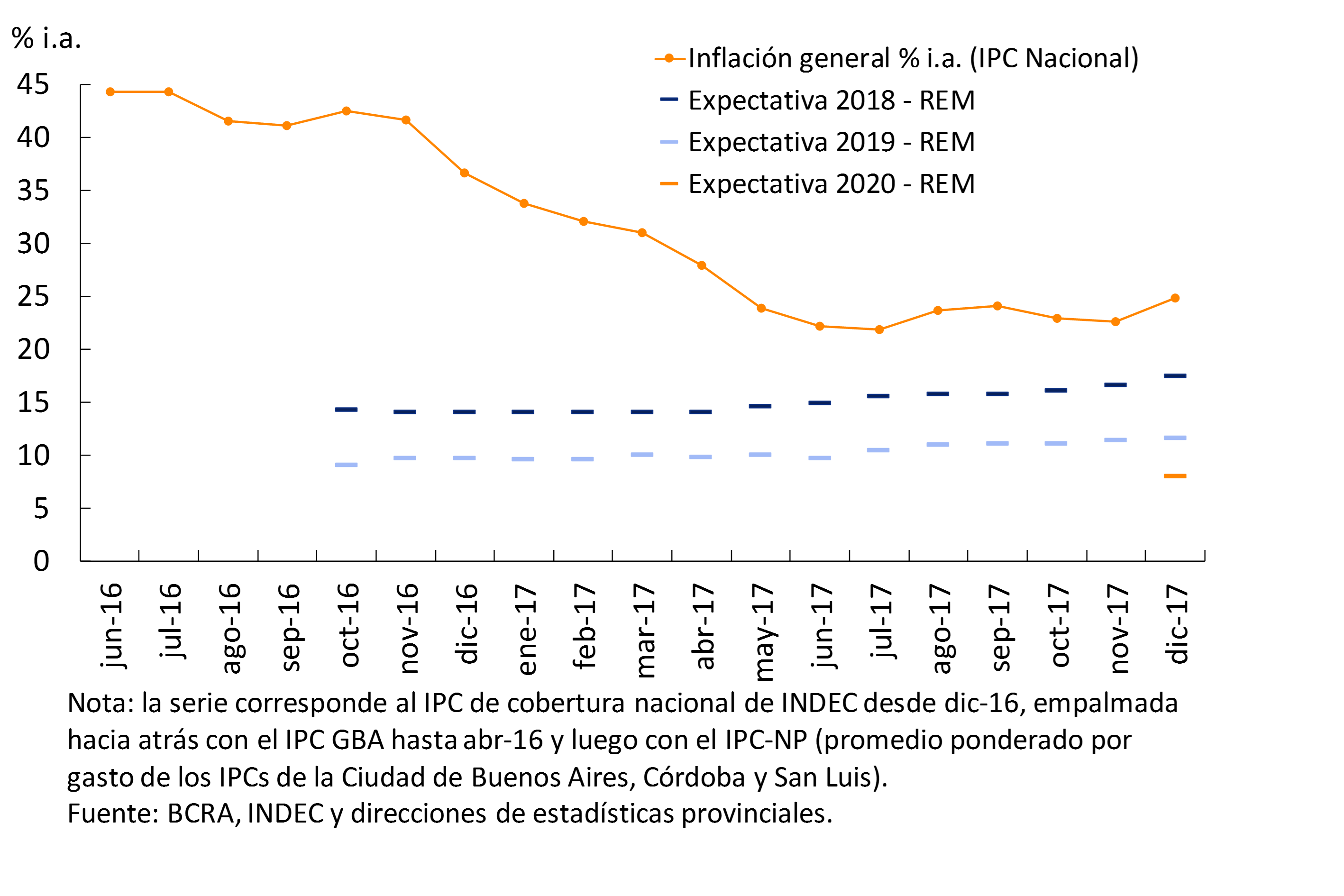
The expectations of market analysts reflect the continuity of the disinflation process. For December 2018, the REM estimates that inflation will stand at 17.4%, 7.4 p.p. below inflation in 2017.
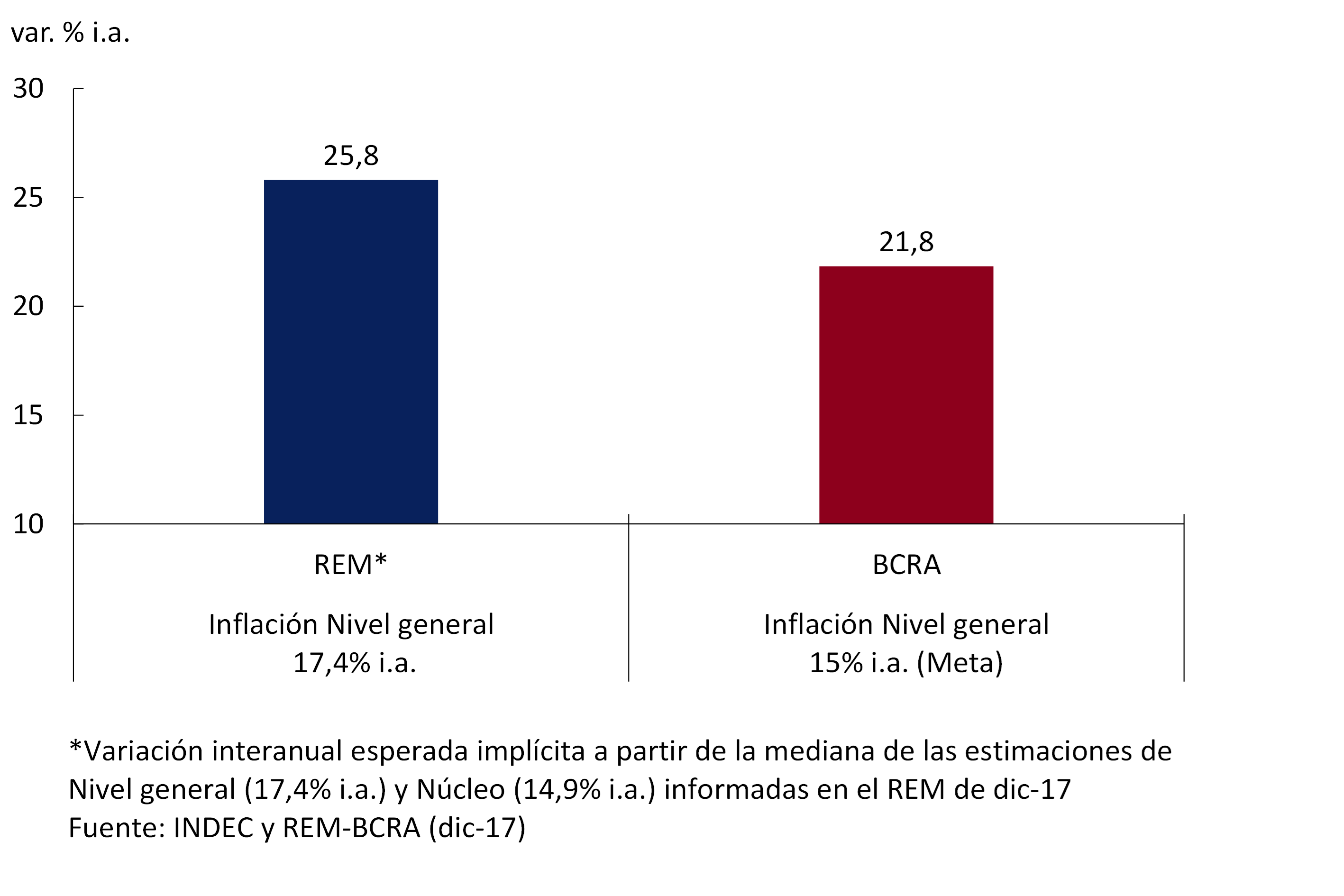
Compared to last September’s survey, expected inflation for 2018-22 rose 1.7 p.p. as a result of a larger-than-expected adjustment in the prices of regulated services. The implicit projection in the REM of the regulated component rose to 25.8% YoY for 2018 (+4.2 p.p. compared to the previous IPOM), while expected core inflation rose 0.9 p.p. to 14.9% YoY.
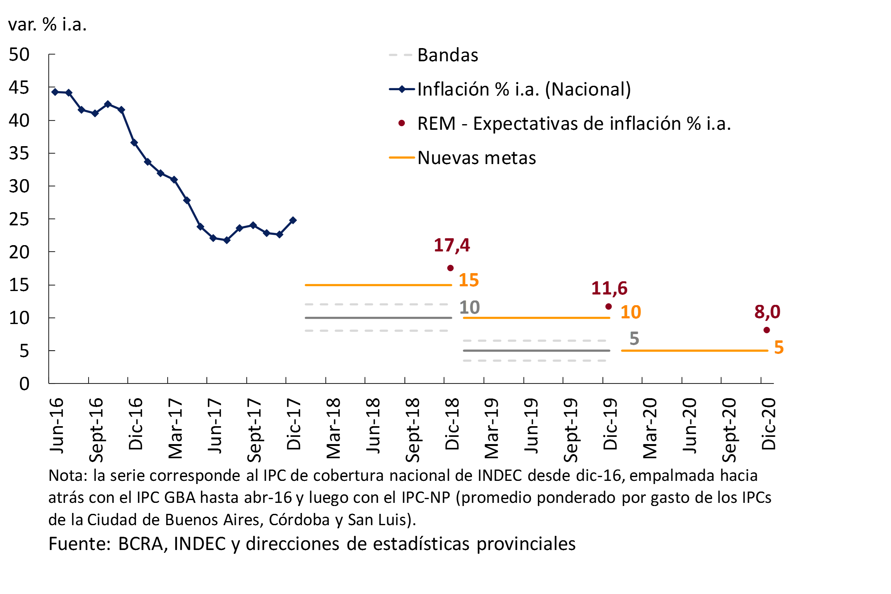
The new inflation target for December 2018 (15% YoY) is within the REM’s expected inflation range (see Figure 4.10). However, the median market forecast is 2.4 p.p. higher than the target. If market forecasts are met, inflation in 2018 would be the lowest in the last nine years.
Figure 4.10 | REM inflation expectations and path compatible with the target
The variation of Regulated Assets implicit in the REM’s projections is above the BCRA’s estimate made based on the information available at present. For utility and transportation rates, there is information from announcements and/or public hearings. For the rest of the items included in the Regulated Items, a trajectory consistent with the goal set for this year is assumed. Using the information described above, the expected increase for regulated in 2018 would be 21.8% YoY (see Figure 4.11).
Figure 4.11 | Regulated Inflation. Implicit in the expectations of the REM and the BCRA’s estimate. December 2018
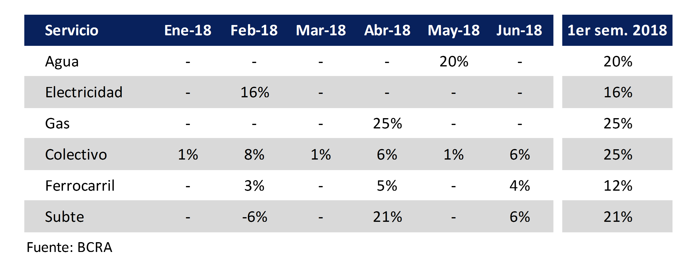
Most of the increases planned for the full year would be concentrated in the first half of the year. Public transport will increase in February, April and June. The first update of public transport coincides with the implementation of the “RED SUBE” system, a scheme that contemplates the application of discounts to integrated trips. Due to the introduction of this new system, the increase that consumers will face will be lower on average (see Section 3 / How much does public transport increase?). Electricity and gas tariffs would have a first adjustment in February and April, respectively (see Table 4.2).
Table 4.1 | Expected increases in regulated services 2018. National CPI
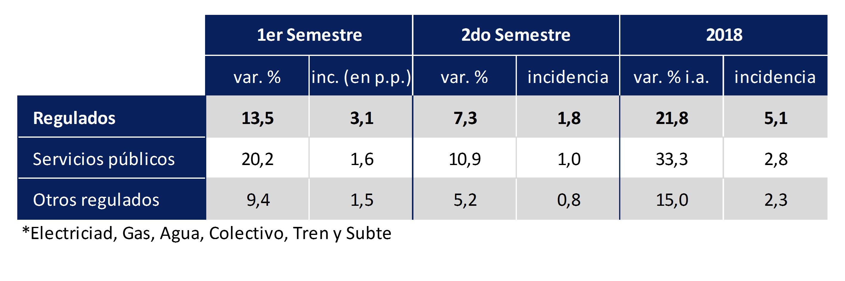
Table 4.2 | Expected increases in regulated services for the first half of 2018. (National CPI; var. % mens.)
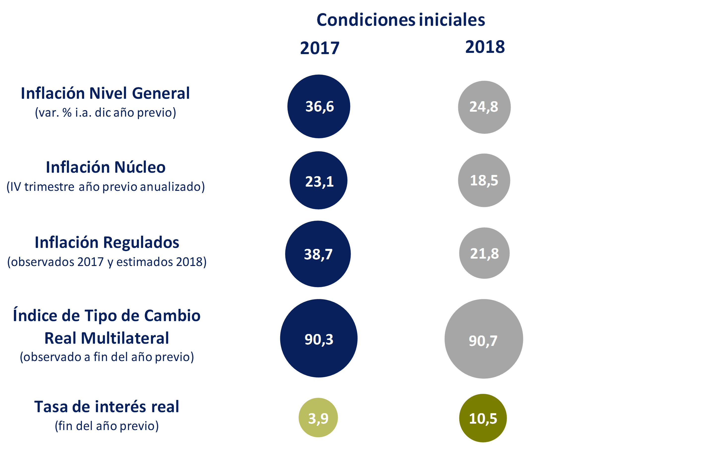
The initial conditions for meeting the inflation target for 2018 are more favorable than those of the previous year. The year-on-year variation of the general level stood at 24.8% in December 2017, 11.8 p.p. below that of 2016; annualized core inflation in the last quarter of 2017 was 18.5% (vs. 23.1% in 2016); the forecast for the adjustment of regulated entities for 2018 is significantly lower than the increase observed in 2017; the Multilateral Real Exchange Rate remained virtually unchanged in 2017 and the monetary policy bias at the end of 2017 is more contractionary than in the same period of the previous year (see Figure 4.12 and Chapter 5. Monetary Policy).
Figure 4.12 | Initial conditions
For 2019 and 2020, the REM forecasts falling inflation of 11.6% YoY and 8% YoY, respectively, in line with the new inflation targets. For 2019, the forecasts are 1.6% p.p. above the target and for 2020, 3 p.p. (see Figure 4.13).
Figure 4.13 | Inflation targets and expectations. 2018-2020
5. Monetary policy
Year-on-year inflation in December 2017 was 24.8%, above the target sought for the year (14.5% ±2.5%). This deviation was explained by a monetary policy that was relaxed in the latter part of 2016 and the first months of 2017, by a higher-than-expected persistence of inflation in nominal contracts, and by a higher-than-expected increase in regulated prices.
The evolution of the inflation rate above what was desired in the first months of last year led the Central Bank to increase the contractionary bias of monetary policy, increasing the policy rate three times, which went from 24.75% in March to 28.75% in December 2017, and actively operating in the secondary LEBAC market to raise the interest rates of these instruments.
The result of these decisions began to be observed in the second half of last year, when the three-month moving average of core inflation pierced the level of 1.7% per month observed until then to close the year at 1.4% per month (18.5% annualized). Likewise, the year-on-year inflation rate registered a fall of 11.8 p.p. in December last year compared to the same month of the previous year, while inflation expectations remained anchored throughout the year and with a clear downward trend for the coming years. Unlike other disinflation processes that have occurred in our country, this time the reduction of inflation is being achieved without delaying tariffs, with free prices and exchange rates, with credit expansion, with growth of the economy and without a sustained real appreciation of the peso.
Given the deviation from the inflation targets observed during the past year, in addition to having increased the contractionary bias of monetary policy, a deferral of the 5% target was announced, defining a new path of 15% for this year, 10% for 2019 and 5% from 2020. In this context, the Central Bank decided at the beginning of January to reduce its monetary policy rate of 75 p.p. to bring it to 28% per year, while LEBAC rates also accommodated the new trajectory of target inflation, showing a fall in the secondary market of between 2 and 3 p.p., according to the deadline, from the maximum levels of the end of December last year. Along with the postponement of the target, the path of transfers from the Central Bank to the National Treasury was announced, which gives greater predictability to monetary policy.
This year’s starting point for inflationary dynamics looks more favorable than at the beginning of last year: a greater initial contractionary bias of monetary policy is observed; a lower expected increase in regulated prices; and lower persistence of inflation. Even so, in the coming months, the Central Bank will be cautious in adapting monetary policy to the new path of disinflation.
5.1 Monetary policy in 2017: accountability
Inflation in December 2017 amounted to 24.8% year-on-year, above the target sought for the year (14.5% ±2.5%) (see Figure 5.1). This deviation was explained by the combination of several factors: a) a monetary policy that was relaxed in the latter part of 2016 and the first months of 2017, when the Central Bank reduced the interest rate in the face of the favorable evolution of inflation in the last months of 2016; b) a persistence of inflation in nominal contracts greater than expected; (c) a higher-than-expected increase in regulated prices.
Figure 5.1 | Inflation and targets in 2017
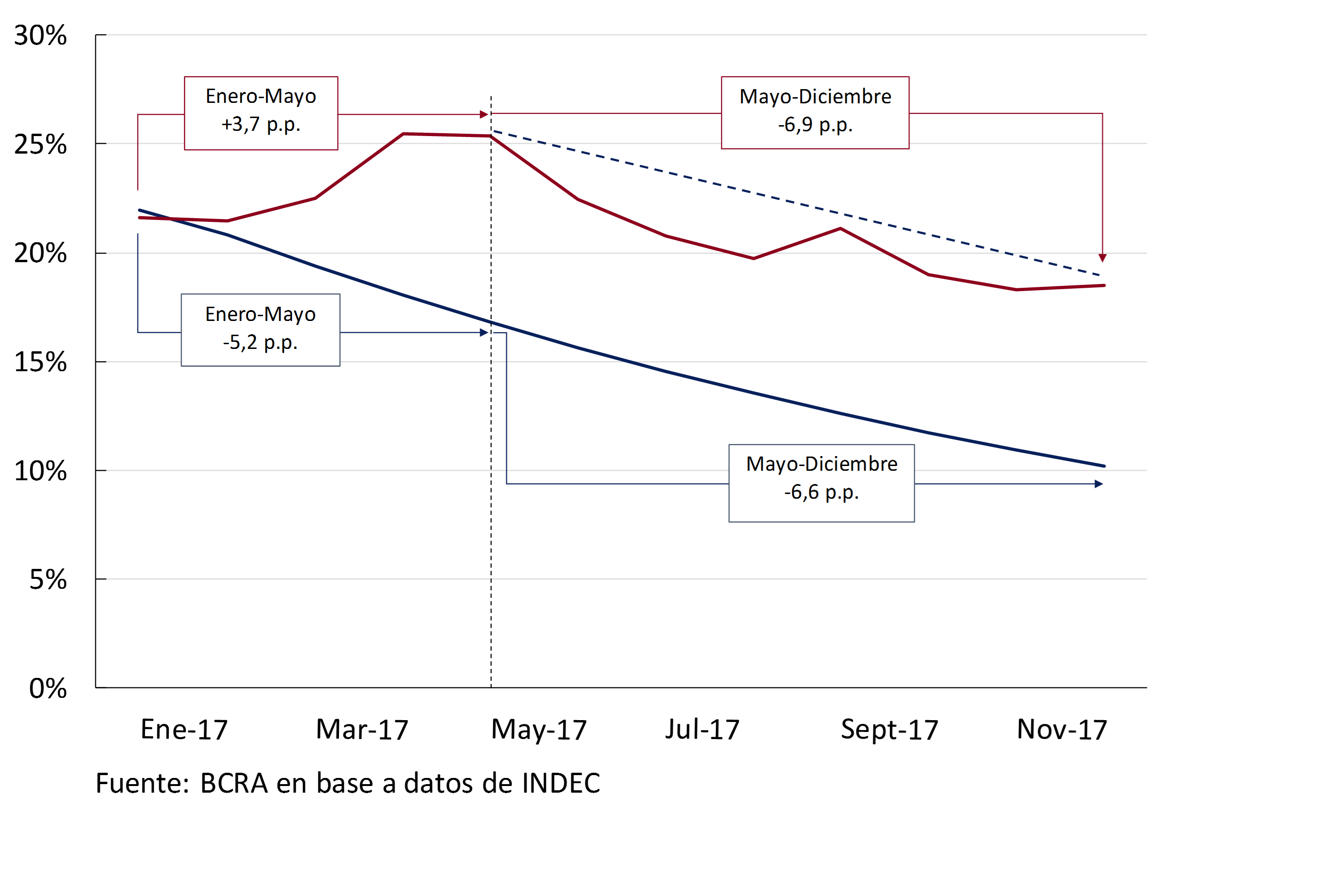
The very favorable performance of inflation in the second half of 2016 had led the Central Bank to excessively relax the bias of monetary policy. This change in monetary policy led to price dynamics in the first half of 2017 that were out of line with the path sought by the monetary authority (see Figure 5.2). In response, as of April last year, the Central Bank increased the contractionary bias of monetary policy by raising the policy rate three times and actively operating in the secondary LEBAC market to increase interest rates on these instruments (see Figure 5.3). Thus, while in the first months of 2017 the trajectory of core inflation deviated from the desired one, since the change in monetary policy the rate of decline in inflation has approached that required to meet the target (see Figure 5.2).
Figure 5.2 | Velocity of disinflation: observed vs. compatible with the target (core inflation; prom. mov. 3 months annualized)

The result of these decisions began to be evident in the second half of 2017, when the three-month moving average of core inflation pierced the level of 1.7% per month observed until then. 23 This indicator showed a significant decline and ended the year at 1.4% per month (18.5% annualized), the lowest value in the last six years (see Figure 5.3). For its part, general inflation fell by 11.8 p.p. in December compared to the year-on-year variation of the same month of the previous year, while inflation expectations remained anchored throughout last year, showing a clear downward trend for the coming years (see Chart 5.4).
Figure 5.3 | Monetary policy bias and inflation
However, inflationary persistence in nominal contracts (e.g., wage agreements) was higher than expected. Many nominal contracts were traded in 2017 with significantly lower increases than those of annual inflation recorded in 2016, showing that the inflation targeting scheme managed to anchor inflation expectations; but these increases were greater than those compatible with the inflation target. Given these persistence mechanisms, monetary policy was less contractionary than it should have been to achieve the inflation target.
Finally, to a lesser extent, an increase in regulated prices above what was expected was another reason for the deviation from the target. In December 2016, the Market Expectations survey expected regulated price inflation to be 29.5% annually, but it turned out to be 38.7%. This factor contributed an additional annual incidence of 1.9% than expected. Within this group, there are higher-than-expected increases in gasoline (0.6%), prepaid medicine services (incidence of 0.4%) and education (0.3%). In this area, there were also higher-than-expected tariff increases (electricity, gas, water and transport), which directly affected companies’ costs and caused an impact on prices in other items.
Figure 5.4 | Anchored inflation expectations
Unlike other disinflation processes that have occurred in our country, this time the reduction in inflation is being achieved without delaying tariffs and with free prices and exchange rates. Likewise, the drop in inflation last year occurred together with a favorable performance of the economy: credit expanded markedly in real terms and the growth of economic activity would approach 3% in 2017, with no signs of slowing down both in the Central Bank’s contemporary prediction indicator (it shows a seasonally adjusted growth rate of 0.94% for the fourth quarter of last year) and in the the leading index calculated by the Central Bank (which is not anticipating a change from the current expansionary phase) (see Section 3.1).
The flexible exchange rate regime, which is common in countries with inflation targets, has allowed disinflation to develop without a sustained real appreciation of the peso. In fact, the multilateral real exchange rate has oscillated since mid-2016 around a level that is 21.5% higher than before the unification of the foreign exchange market at the end of 2015 (see Figure 5.5). This dynamic differs from the episodes of systematic real appreciation of the domestic currency characteristic of stabilization programs based on the fixing of the exchange rate. Having a floating exchange rate allows the economy to better absorb external shocks and helps to avoid the accumulation of macroeconomic imbalances. 24
Figure 5.5 | Multilateral Real Exchange Rate
Given the deviation from the inflation targets observed during the past year, in addition to having increased the contractionary bias of monetary policy, a deferral of the target of 5% from the original path announced was announced; new goals are defined of 15% for this year, 10% for 2019 and 5% from 2020. The new targets are consistent with the declining trend in inflation expectations and remain below the inflation forecast by the market, which according to the REM of December last year are 17.4% for 2018, 11.8% for 2019 and 8% for 2020 (see Figure 5.6).
Figure 5.6 | Inflation, Targets and Expectations 2018-2020
The interest rates registered until the deferral of the target were in line with the objective of reaching inflation of 10% (±2%) during this year. At the same time, in the Central Bank’s view, the disinflation process has been on track over the last six months, with core inflation in the last three months at around 18% in annualized terms. On the other hand, the impact of December’s increase in regulated prices on core inflation was limited and is interpreted as a temporary phenomenon on the inflation rate.
In this context, on January 9 the Central Bank decided to reduce its monetary policy rate by 75 p.p. to bring it to 28% per year. Meanwhile, LEBAC rates also accommodated the new path of target inflation, showing a fall in the secondary market between 2 and 3 p.p., depending on the term, from the maximum levels of late December last year (see Figure 5.7). Based on the favorable evolution of core inflation and the deferral of the inflation target, this reduction in the benchmark interest rate prevents the real interest rate from increasing and, therefore, the contractionary bias of monetary policy.
Figure 5.7 | Yield curve of LEBACs in the secondary market
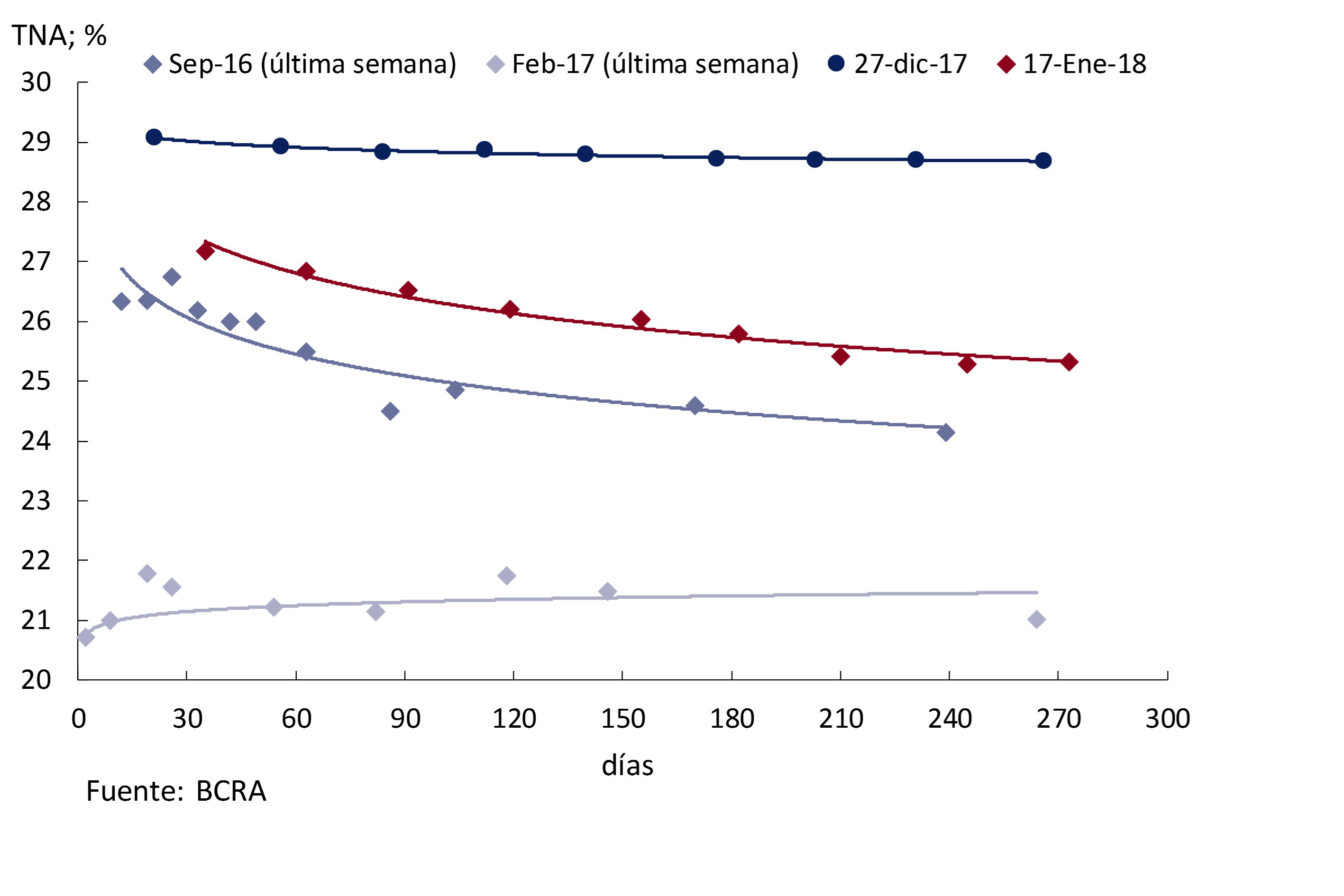
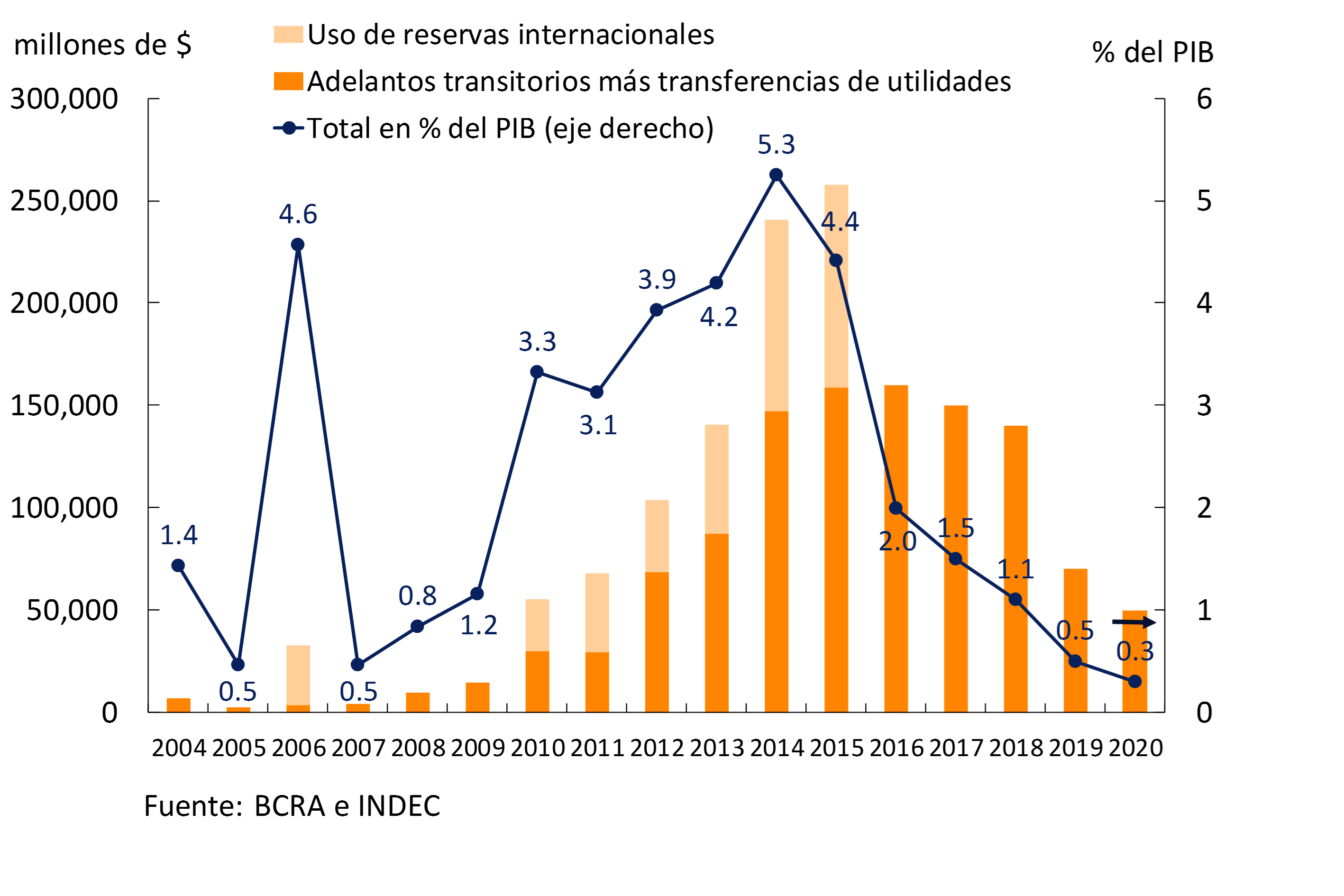
Along with the postponement of the target, the path of transfers from the Central Bank to the National Treasury was clarified, in order to provide greater predictability to the management of monetary policy. The National Public Sector Budget for this year included a transfer of funds of $ 140,000 million or 1.1% of GDP, which showed a decrease of 0.4% of GDP compared to the amount granted in 2016 (see Figure 5.8). In line with the planned gradual correction for the fiscal deficit, a reduction in transfers was defined at $70 billion or 0.5% of GDP in 2019 and, for 2020 onwards, a level related to the increase in demand for money associated with the real growth of the economy. Assuming a monetary base stock of 10% of GDP and a growth of the economy of 3%, by 2020 the transfer of funds to the Treasury would reach 0.3% of GDP. Thus, given the interest rate and the demand for money, a downward trend in these transfers implies a lower issuance of non-monetary liabilities by the Central Bank for the same foreign exchange purchase path (see Section 5 / The sustainability of LEBACs, for an analysis of the impact of this transfer path on the Central Bank’s balance sheet).
Figure 5.8 | Transfers from the Central Bank to the National Treasury
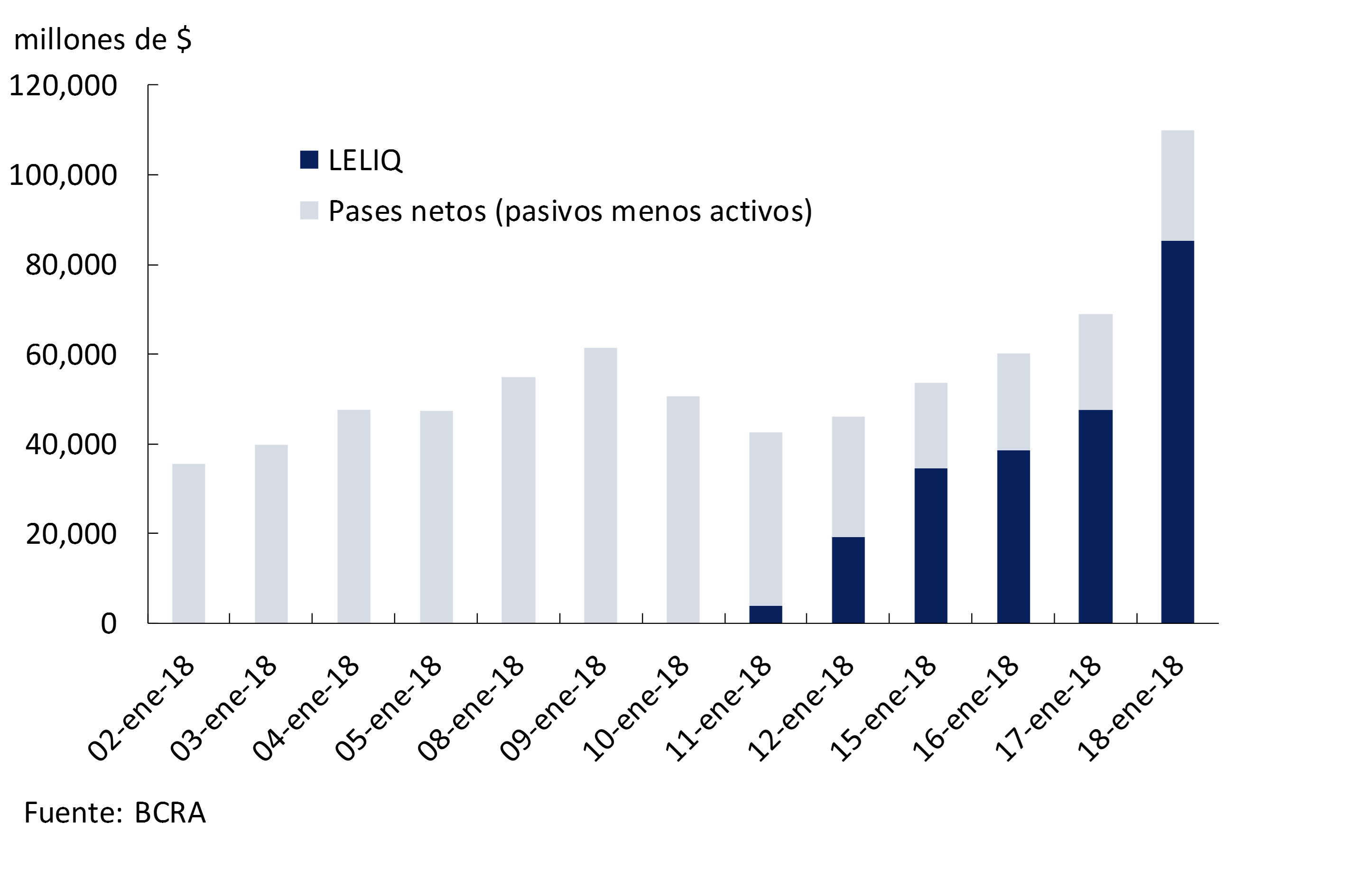
At the beginning of 2018, the Central Bank implemented the Liquidity Bills (LELIQ). 25 These bills are peso-denominated instruments with a maturity of seven days. The monetary authority offers the LELIQ on a daily basis only to financial institutions for its own portfolio. Likewise, they can be traded on the secondary market only between financial institutions and can also be used as collateral in pass operations. The objective of these new monetary regulation instruments is to improve the implementation of monetary policy through an improvement of the pass market. Banks are given a paper that can be traded in the secondary market – which will give greater liquidity to the interbank funds market for up to seven days – and whose interest rate will be linked to the policy rate corridor. Since their implementation, these instruments have gained share over passes in the holdings of financial institutions (see Figure 5.9).
Figure 5.9 | Recent developments in LELIQ and net passes
This year’s starting point for inflationary dynamics looks more favorable than at the beginning of last year (see Figure 4.12). First, core inflation, measured as the three-month monthly average, was below the record for the same period in 2016 in December last year (18.5% versus 23.1%); Meanwhile, year-on-year general inflation in December 2017 was 24.8% compared to 36.6% in the same month of the previous year, which is favorable given the persistence that is still observed in the formation of contracts. Likewise, the increase in regulated prices expected for this year would be substantially lower than that observed last year (21.8% versus 38.7%). Finally, the bias of monetary policy at the end of 2017, measured by the level of the real interest rate of monetary policy, is more contractionary than that recorded at the end of 2016 (10.5% per year versus 3.9% per year). Even so, in the coming months, the Central Bank will be cautious in adapting monetary policy to the new path of disinflation.
5.2 Increase in the contractionary bias of monetary policy in 2017
The inflation targeting scheme requires both the explanation of the deviation and the measures implemented to return inflation to a path in line with the target. Below is a review of the main measures taken by the Central Bank to increase the contractionary bias of monetary policy during 2017, from the moment it was observed that the dynamics of inflation deviated from that sought.
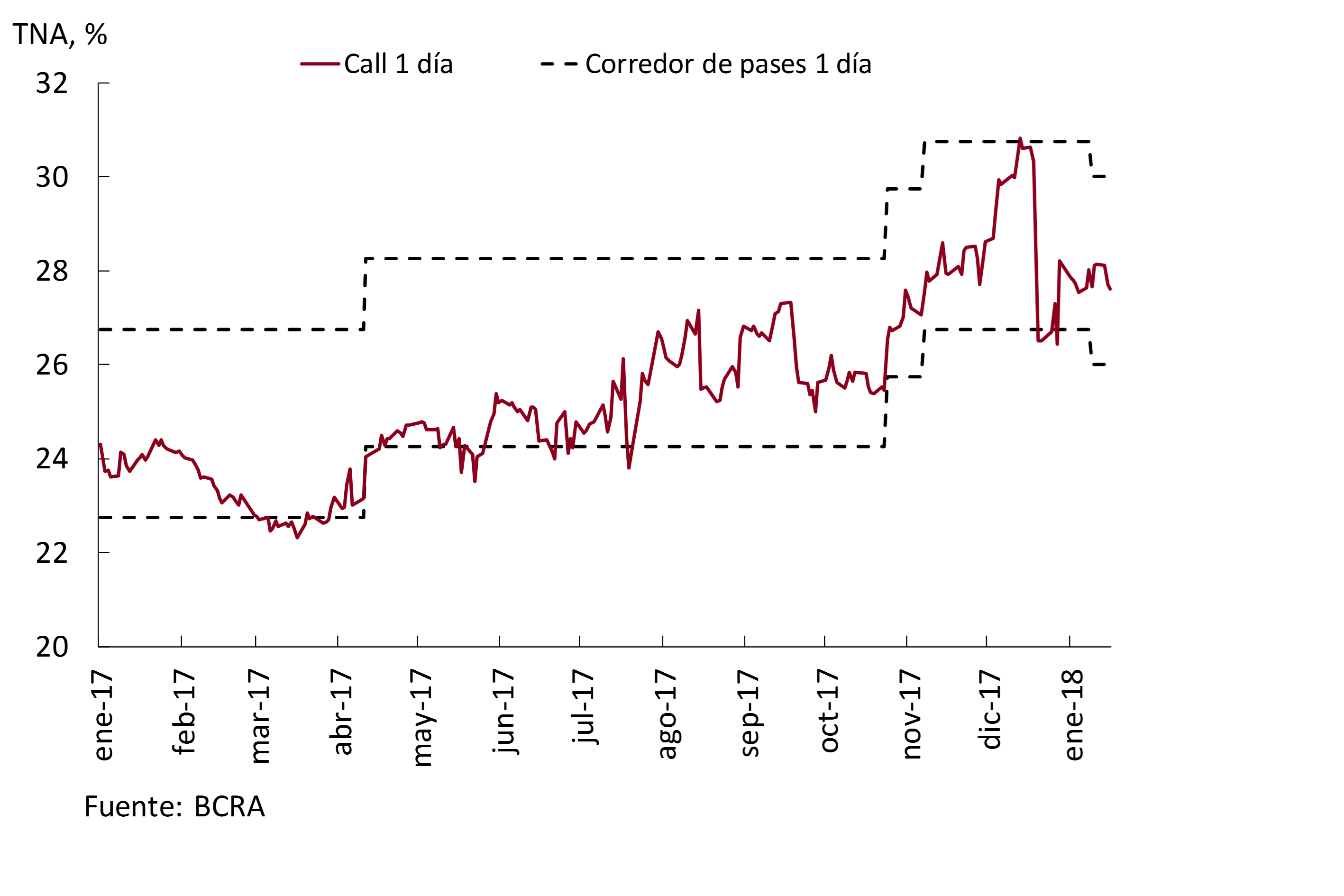
The increase in monthly headline inflation and the persistence of core inflation in the first months of last year led the central bank to increase the policy interest rate (the center of the 7-day pass corridor) by 150 basis points in April, another 150 basis points in October, and an additional 100 basis points in November (see Figure 5.10). Thus, the policy rate went from 24.75% per year in March to 28.75% per year in December, which brought the real policy interest rate from 5% per year to about 10% per year in the same period (see Figure 5.3). 26
Figure 5.10 | Pass and Call Rate Broker (1 day)
In addition to the management of the policy interest rate, the Central Bank affected the liquidity conditions of the LEBAC secondary market through open market operations over the past year, in order to reinforce the transmission of its policy interest rate to the rest of the economy’s interest rates. The monetary authority made sales of securities for VN $ 1,127,829 million during 2017, which represented 20% of the total operations carried out in the secondary market of LEBAC. Thus, the yield curve of Central Bank securities increased throughout the year, with increases of around 7.5 p.p. between the end of February and December 27 last year (see Figure 5.11).
Figure 5.11 | Yield curve of LEBACs in the secondary market
Money market interest rates followed the rise in the monetary policy rate and the LEBACs and remained limited within the pass corridor (mainly from July onwards). Let us remember that the interest rate of passive passes acts as a floor for the interest rates of the interbank market: when the market rate is pressured to be below the floor, agents can place their excess funds by making passive passes with the Central Bank. While the interest rate on active passes works as a ceiling: when the market rate faces pressure to move above the ceiling, agents can cover their shortfall in funds with loans from the Central Bank through active passes. Thus, both the rate of passes between third parties and the rate of 1-day interbank calls increased by about 6 p.p. between March and December to close the year at a monthly average of 27.7% annually and 28.8% annually, respectively (see Figure 5.10).
5.3 The expansion of lending put pressure on banks’ liquidity and passive interest rates, reinforcing the policy rate transmission mechanism
Private sector deposits in pesos grew at a real monthly rate of 0.3% without seasonality during 2017, accumulating an expansion of 4% year-on-year in December. Demand placements (current account and savings account) showed a better performance, with a monthly increase of 0.7% in real terms without seasonality, compared to fixed-term deposits, which remained practically stagnant in the year. In the last quarter of the year, deposits were more dynamic, with a real monthly increase of 1.5% without seasonality, driven mainly by fixed-term deposits, which grew at a rate of 2.0% monthly, while demand loans increased by 1.1% month-on-month (see Figure 5.12).
Figure 5.12 | Evolution of loans and deposits (from the private sector in pesos) (without seasonality)
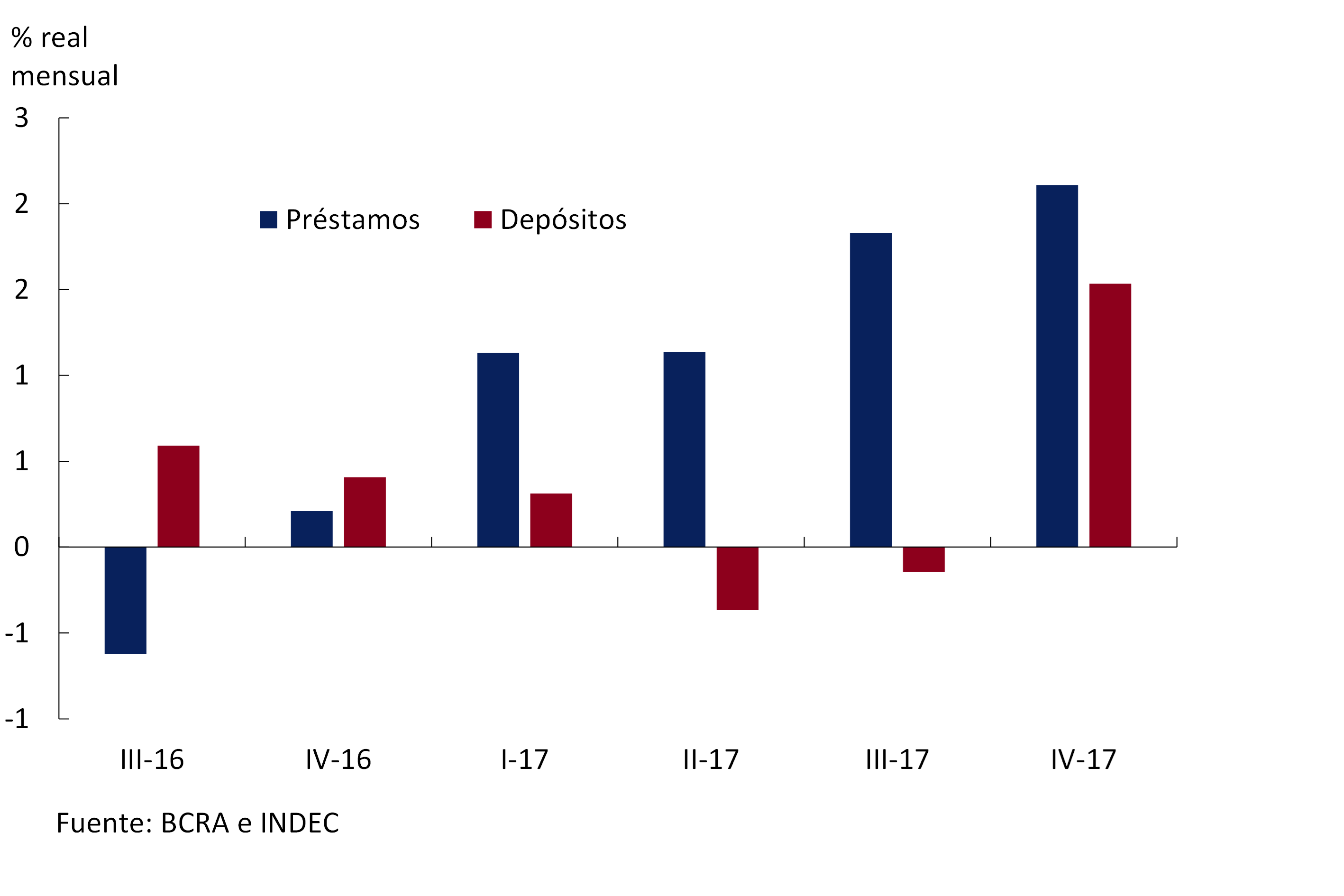
Lending expanded at a faster rate than deposits (see Figure 5.12). Thus, loans in pesos to the private sector increased 1.6% month-on-month without seasonality throughout the year, reaching an expansion of 20.3% real year-on-year in December (an increase of 24.3% real year-on-year if loans in foreign currency are also considered). Although increases were observed in most of the lines, the largest increases were registered in mortgage credit, within which UVA loans stood out – with a 92% share of disbursements in the case of individuals in December – in pledges, in personal loans and in documents. Despite this dynamic, the stock of loans to the private sector in terms of GDP is still low both in historical terms and in relation to other emerging economies (11.1% of GDP for financing in pesos and 13.4% of GDP when loans in foreign currency are also considered) and therefore has growth potential (see Figure 5.13).
Figure 5.13 | Loans to the private sector as % of GDP

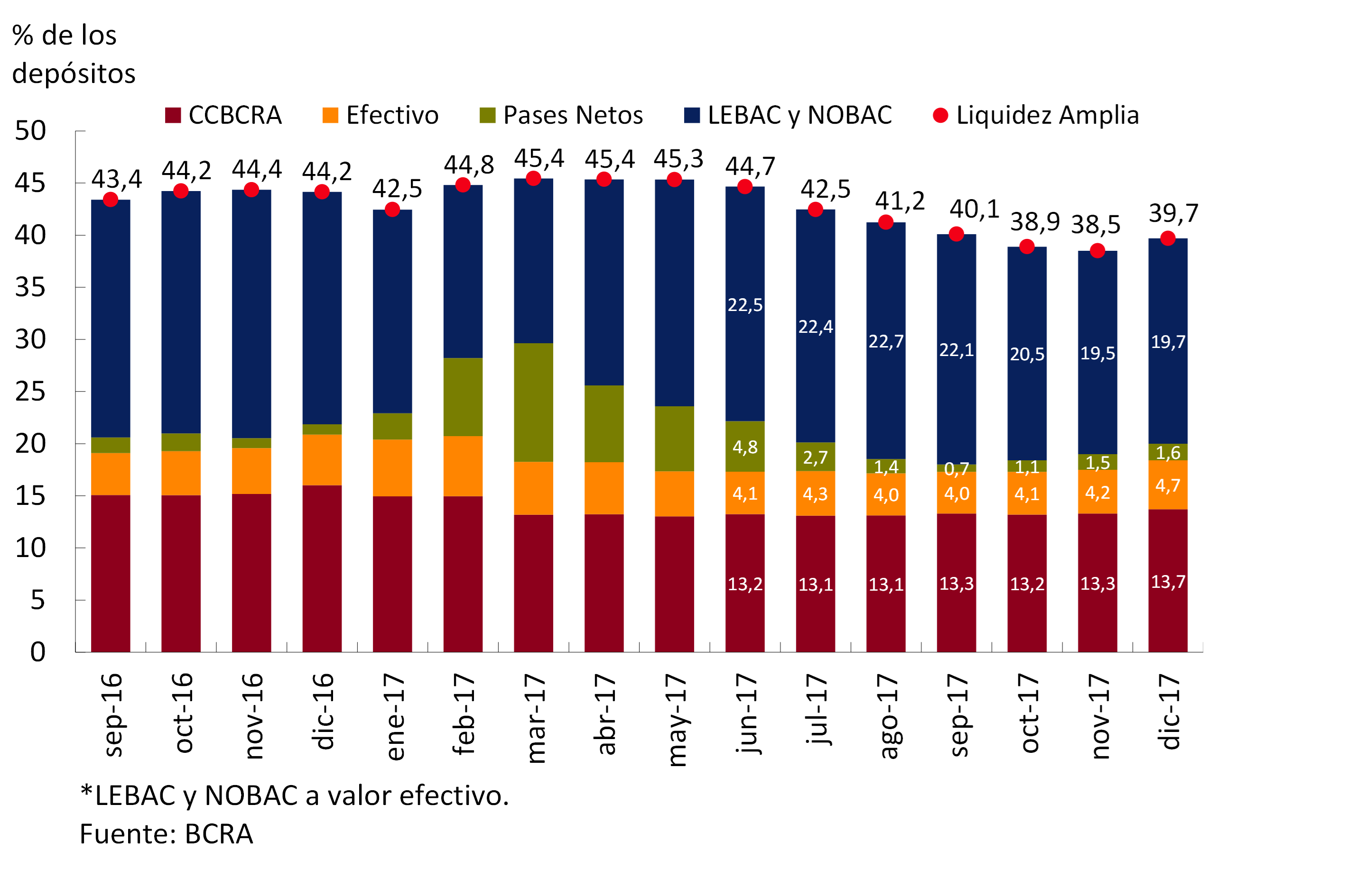
In a context in which the granting of loans to the private sector exceeded the growth of deposits, the liquidity of financial institutions in the segment in domestic currency decreased. Total liquidity, which includes cash in banks, current account deposits at the Central Bank, LEBAC and net passes, fell from 45.4% of deposits in March to 39.7% in December, while excess liquidity (taking only LEBAC and net passes) went from 27.2% of deposits to 21.3% in the same period (see Figure 5.14). This helped to strengthen the mechanism for passing through policy rates to passive interest rates in the financial system.
Figure 5.14 | Liquidity ratio of financial institutions
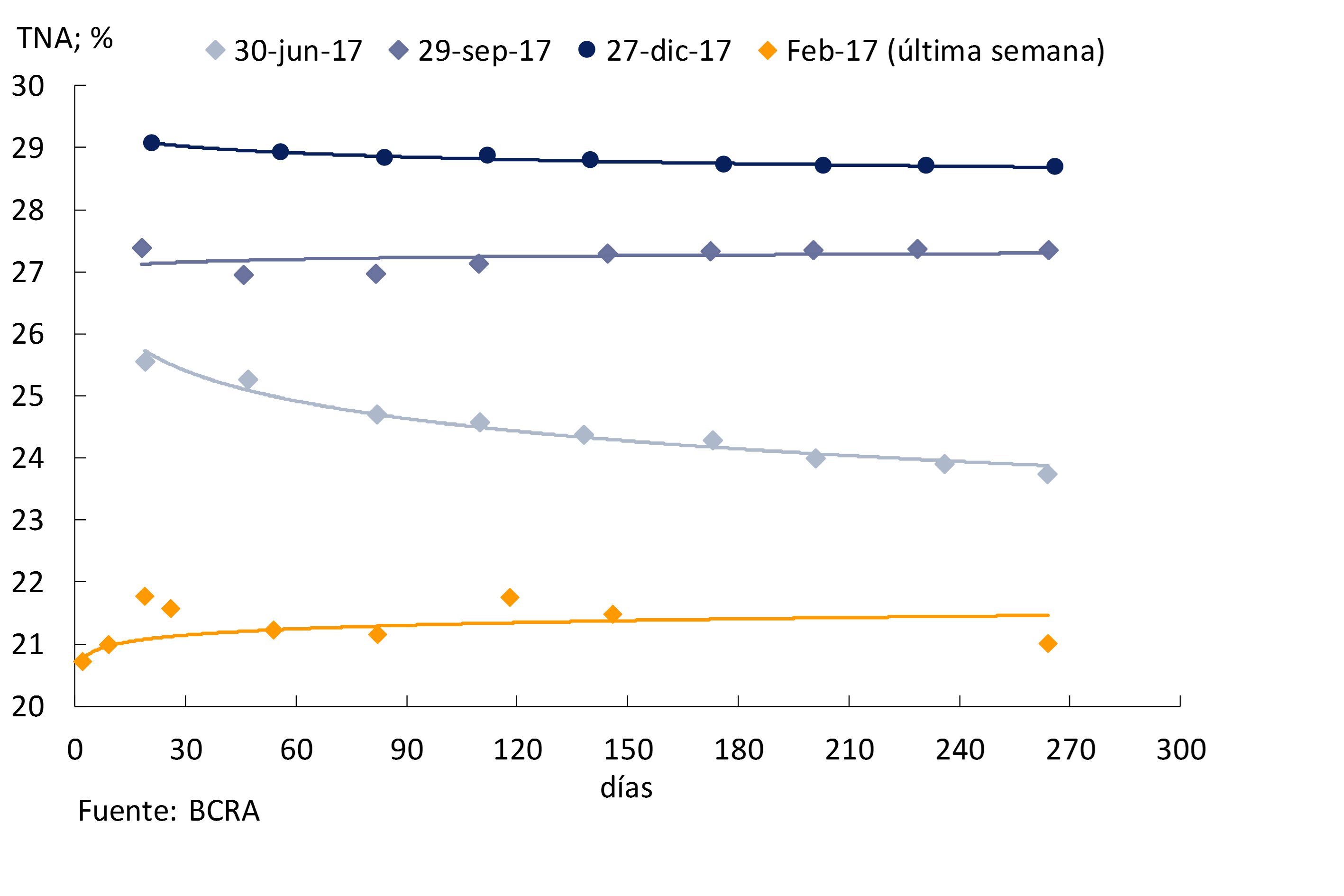
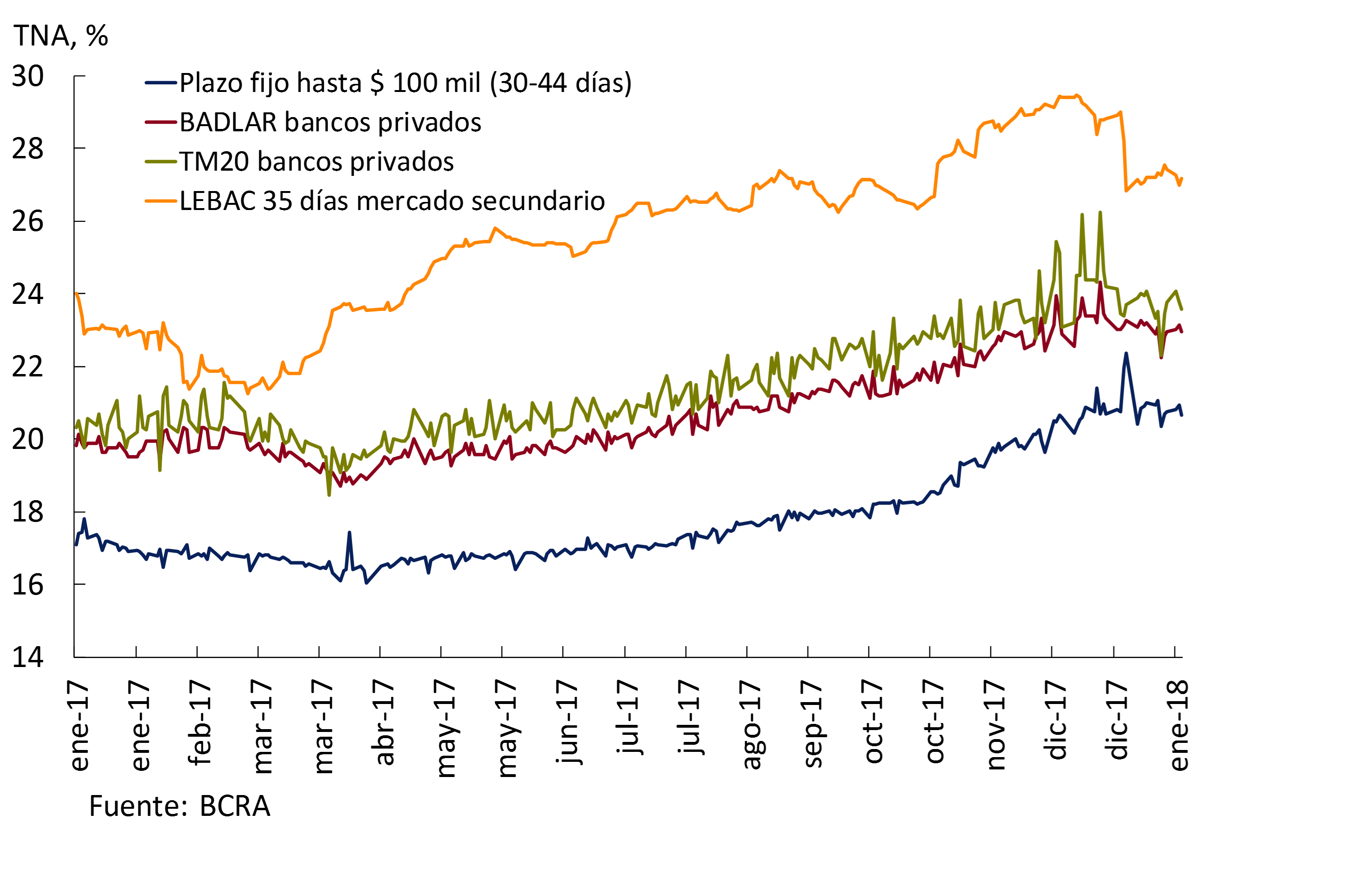
As a result, interest rates on deposits began to increase starting in April, at first slowly, then with increasing increases as the year progressed. In the wholesale segment, the BADLAR rate of private banks increased 3.7 p.p. since March to reach a monthly average of 23.2% in December, while in the retail segment, the increase in the interest rate on fixed-term deposits was 4.2 p.p. in the same period, to close December with a monthly average of 20.8% (see Figure 5.15). Interest rates on UVA-adjusted deposits also increased last year, with an average increase of 4 p.p. – an increase that occurred mainly in the second part of the year – to reach a monthly average of 5% per year in the last month of last year.
Figure 5.15 | Bank Passive Interest Rates
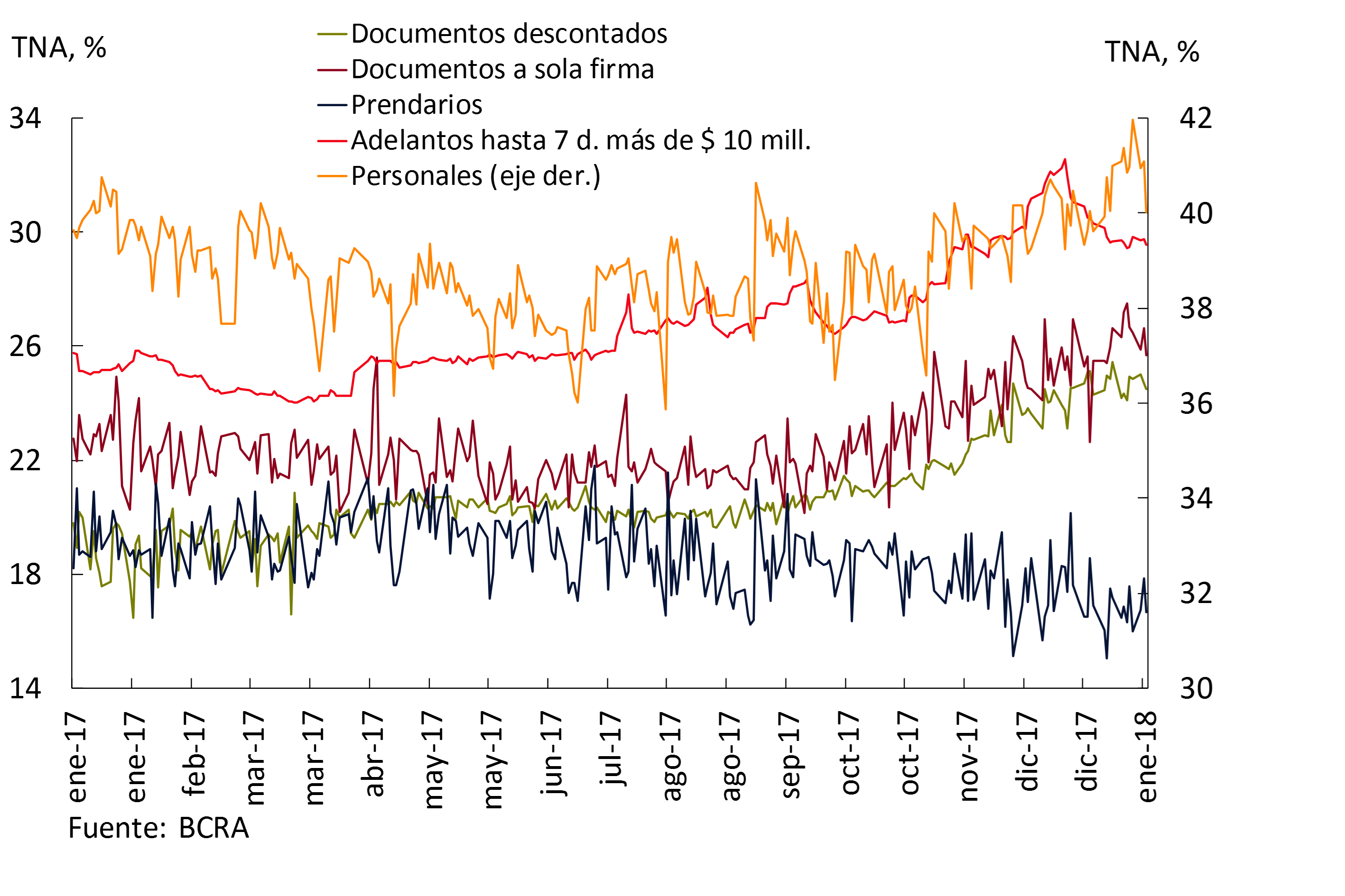
On the other hand, lending rates showed a mixed behavior throughout the year. Interest rates for financing companies increased by magnitudes similar to interest rates on fixed-term deposits, although the increases were mainly concentrated in the last quarter of the year. Thus, the average monthly interest rates on current account advances, single-signature documents and discounted documents registered increases of 4.4 p.p., 3.1 p.p. and 5 p.p. between March and December, respectively (closing at 34.1%, 25.4% and 24.2% annually, respectively in December). Interest rates on loans associated with household consumption increased by a lesser magnitude: the cost of financing personal loans increased 1 p.p. in the same period (up to 40% annually in December), while credit card rates remained practically stable (42.2% annually in December). Finally, the cost of collateral loans fell by 1.3 p.p. between March and December of last year to reach 17.4% annually at the end of the year (see Figure 5.16). UVA-adjusted loan rates also showed heterogeneous behaviors, with the cost of mortgage and pledge loans practically unchanged between March and December (closing the year at around 5% and 10% per year, respectively) and rising 1.7 p.p. in the same period in the case of personal loans to reach 10% per year in the last month of 2017.
Figure 5.16 | Bank lending rates
5.4 The Central Bank continued to accumulate international reserves
In 2017, the Central Bank continued to accumulate foreign currency with the purpose of reaching a level of international reserves similar to that of other countries in the region that also operate with inflation and floating exchange rate targets. On April 18 last year, the monetary authority announced its intention to increase the ratio of international reserves to 15% of GDP. This objective is subordinate to achieving low and stable inflation, and does not have a defined timeline for compliance. This strategy is based on a precautionary demand for foreign currency that does not have the objective of fixing its level but rather to avoid disruptive volatility of the exchange rate. Having an adequate stock of international reserves is part of the BCRA’s macroprudential approach and helps to prevent adverse repercussions on the economy in the face of changes in international liquidity conditions.
Figure 5.17 | Purchases of international reserves by the Central Bank
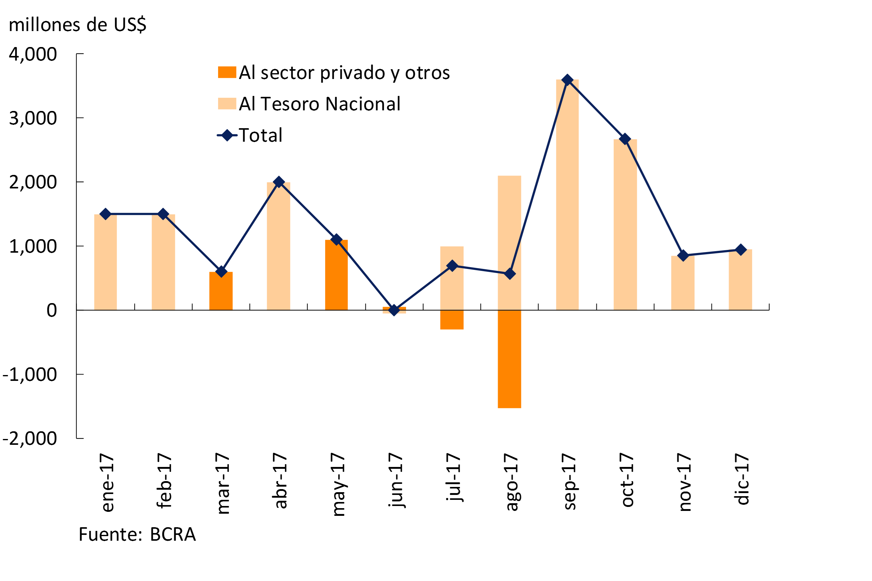
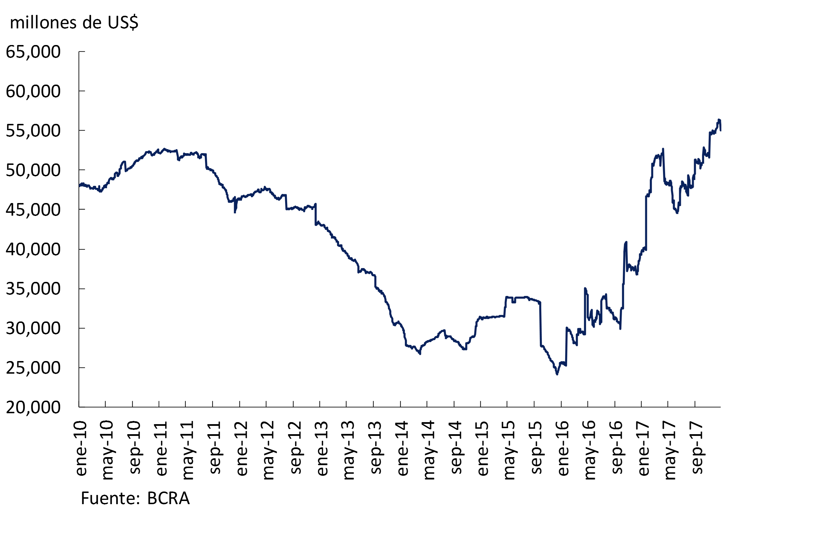
Throughout the year, foreign currency held by the Central Bank increased by US$ 15,747 million, mainly due to direct purchases from the National Treasury, reaching a level of US$ 55,055 million at the end of December (9.1% of GDP), and accumulating an increase of US$ 29,440 million since the end of November 2015 (see Figures 5.17 and 5.18) (see Section 5 / The sustainability of LEBACs for an analysis of the impact of the accumulation of international reserves on the Central Bank’s balance sheet).
Figure 5.18 | Central Bank International Reserve Stock
Section 1 / Impact of structural reforms on productive sectors
During the period 2011-2015, the supply constraints of the Argentine economy became evident with a GDP that showed high volatility around a stagnant trend while labor productivity had a marked decline.
Since the end of 2015, the Government has adopted important measures that could be classified into two axes: the correction of macroeconomic imbalances, and the beginning of a process of structural reforms aimed at sustaining growth in the coming years.
The economic literature shows that structural reforms can have a significant impact on productivity and GDP growth in the long term through different channels that operate on supply (Blanchard and Giavazzi, 2001; Alesina et al., 2005).
The first results of the macroeconomic corrections are the expansion of the economy at an average rate of 4% per year since mid-2016 with increases in employment and a growing contribution from investment. With the aim of consolidating and sustaining the process of economic growth, in December 2017, the Government sent to Congress a series of tax reforms aimed at improving competitiveness by favoring the creation of registered employment, investment and exports. In addition to the tax reform law, there are tax agreements with the provinces that aim to reduce distortionary taxes. 27
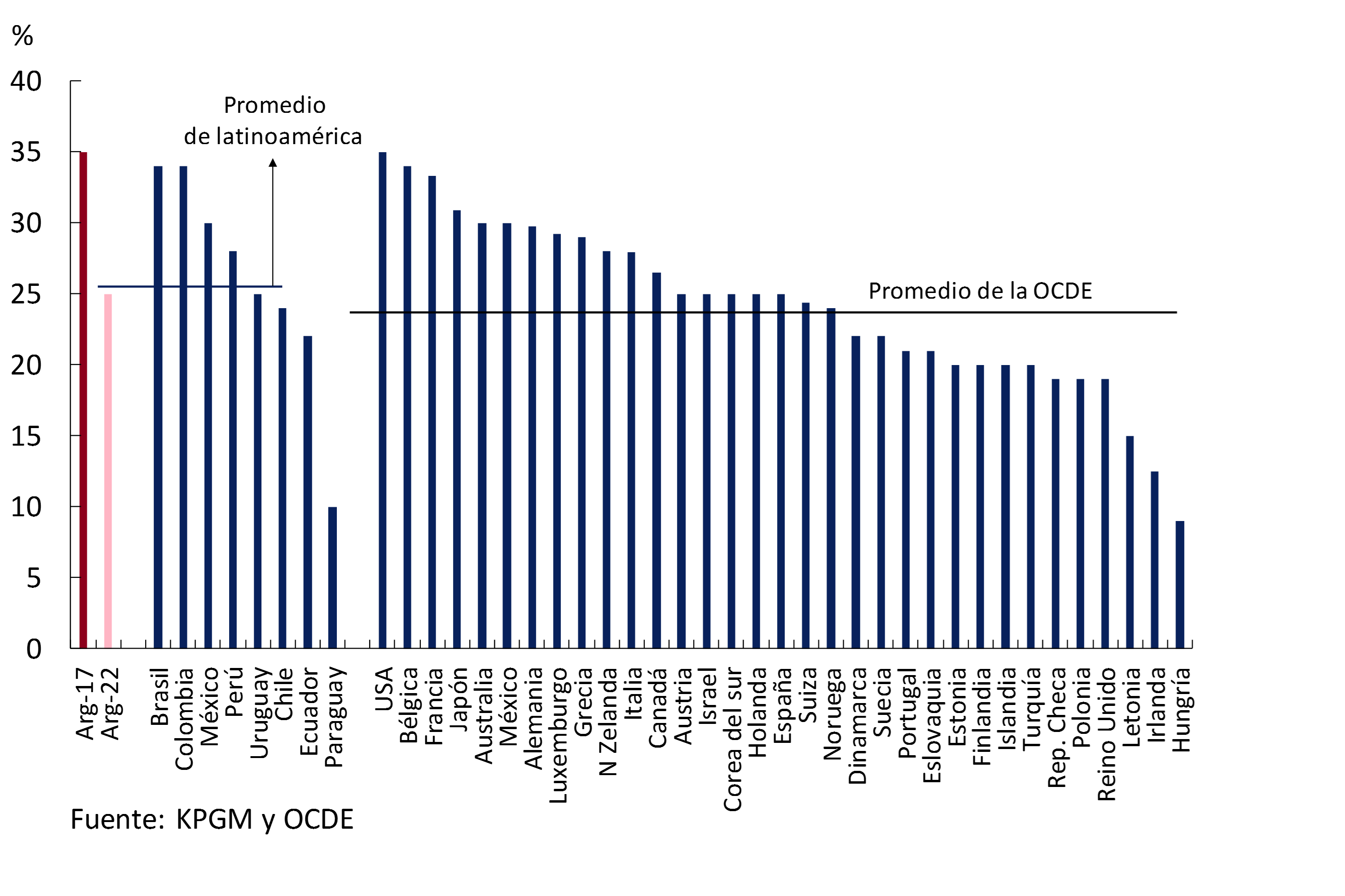
Graph 1 | Total Tax Wedge in Latin America
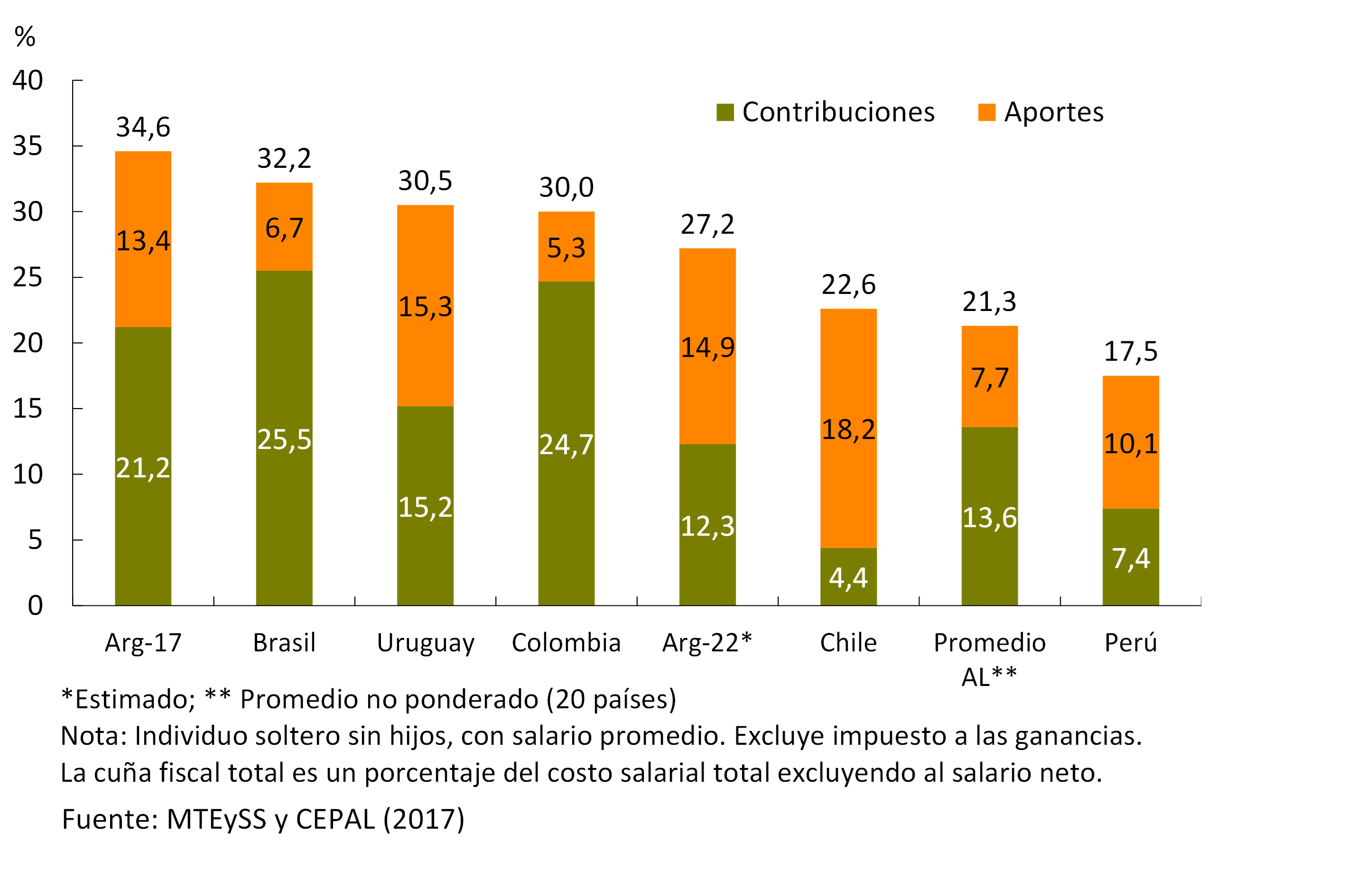
Among the most important points of the tax reform, the establishment of an increasing non-taxable minimum for employer contributions that reduces non-wage labor costs by 7.4 p.p. for 2022 stands out (see Graph 1). This measure practically implies the elimination of the tax for the salaries of the lower deciles, favoring the reduction of informality.
Other relevant points of the tax reform are the reduction of the corporate income tax rate for the reinvestment of profits (see Graph 2), the reduction of the term for the refund of VAT and the payment on account of profits of the tax on checks. The reduction of the tax on legal entities would improve Argentina’s position in the ranking of countries with the lowest rates for companies, favoring the attraction of investments in the country.
Finally, the agreement between the Nation and the Provinces28 shows the commitment to gradually reduce the burden of the Gross Income Tax, which is highly distorting in the production process29. In addition, the provinces undertook to immediately eliminate differential treatments based on the place of establishment, the location of the taxpayer’s establishment or the place of production of the good.
Graph 2 | Corporate Tax Wedge Latin America and OECD
The adoption of structural reforms and their impact on the economy are medium- and long-term processes that are essential to achieve sustained GDP per capita growth rates 30.
Section 2 / The Product Gap: A Small Multivariate Model
Section 2 / The Product Gap: A Small Multivariate Model
Potential output and the output gap are variables of particular interest to central banks. In particular, the output gap is informative about the cyclical conditions of the economy and the possible presence of both inflationary and deflationary pressures.
In both cases, these are unobservable variables that can be estimated using various methodologies, from methods based on the estimation of a production function to different statistical filters. At the same time, it is possible to differentiate two notions of potential product. One of them refers to the productive capacity of the economy in the absence of transitory shocks and full use of resources. Albagli and Naudon (2015) call this measure a trend product. Associated with this concept, the Central Bank currently uses the method of the production function. In a shorter term horizon, the potential output would be that consisting of stable inflation31. In this case, the potential product is usually estimated using univariate filters such as the Hodrick-Prescott (HP) filter, as well as the frequency filters in the Baxter-King and Christiano-Fitzegald versions. Recently, the use of filters or multivariate models, with varying degrees of complexity and structure, has become widespread. The following describes and estimates a multivariate filter for Argentina – on an annual basis in the 1993-2017 interval – using the methodology developed by Benes et al. (2010), which has been adopted with some variations by several central banks and various international organizations32.
The model is estimated with Bayesian methods (which combine a priori assumptions and data analysis) and using the Kalman filter33. Thus, a vector of data of observable variables (which include GDP, unemployment and inflation34) is broken down into its (unobservable) components: trend and cycle. The result is the potential output, the output gap, the potential growth, the unemployment rate consistent with stable inflation (or NAIRU35), and the unemployment gap (understood as the difference between the NAIRU and the effective unemployment rate).
The structure of the model comprises three groups of equations. The former describe the behavior of the product, the determination of the gap and the potential product. Secondly, the Phillips curve is incorporated, which describes the dynamics of inflation, which depends on the output gap and expectations about future inflation, and a backward-looking component is also incorporated. Finally, a third set of equations describes the labor market: the unemployment gap and its relationship to the output gap.
GDP and growth:
y_t=Y_t-overline{Y_{t}}
overline{Y_{t}}=Y_{t-1}+G_t+epsilon_t^overline{Y}
G_t=0.15G^{SS}+0.85G_{t-1}+epsilon_t^G
y_t=0.41y_{t-1}+epsilon_t^y
Phillips curve:
pi_t=0.5pi_{t-1}+0.5pi_{t+1}+0.32y_t+epsilon_t^pi
Labor market:
u_t=overline-U_t{U_t}
overline{U_t}=(0,10overline{U}^{SS}+0,90 overline{U}_{t-1})+U ̅_t^G+ε_t^U ̅
overline{U}_t^G=0.92overline{U}_{t-1}^G+epsilon_t^overline{U}^{G}
u_t=0.23u_{t-1}+0.48y_t+epsilon_t^u
Where y_t is the output gap, Y_t the level of GDP (in logarithms), overline{Y_t} the level of potential output (in logarithms), G_t the potential growth rate, G^{SS} steady-state growth, u_t the unemployment gap, overline{U}_t the NAIRU unemployment rate, U_t the unemployment rate, overline{U}^{SS} the steady-stage unemployment rate, and overline{U}_t^the{G} variation in the NAIRU trend. In turn, six possible types of shocks are defined: to the level of potential output epsilon_t^overline{Y}, to the potential growth rate epsilon_t^G, to the output gap epsilon_t^y, to inflation epsilon_t^pi, to the NAIRU epsilon_t^overline{U}, to the NAIRU trend epsilon_t^overline{U}^{G} and to the unemployment gap epsilon_t^u.
Graph 1 | Product gap
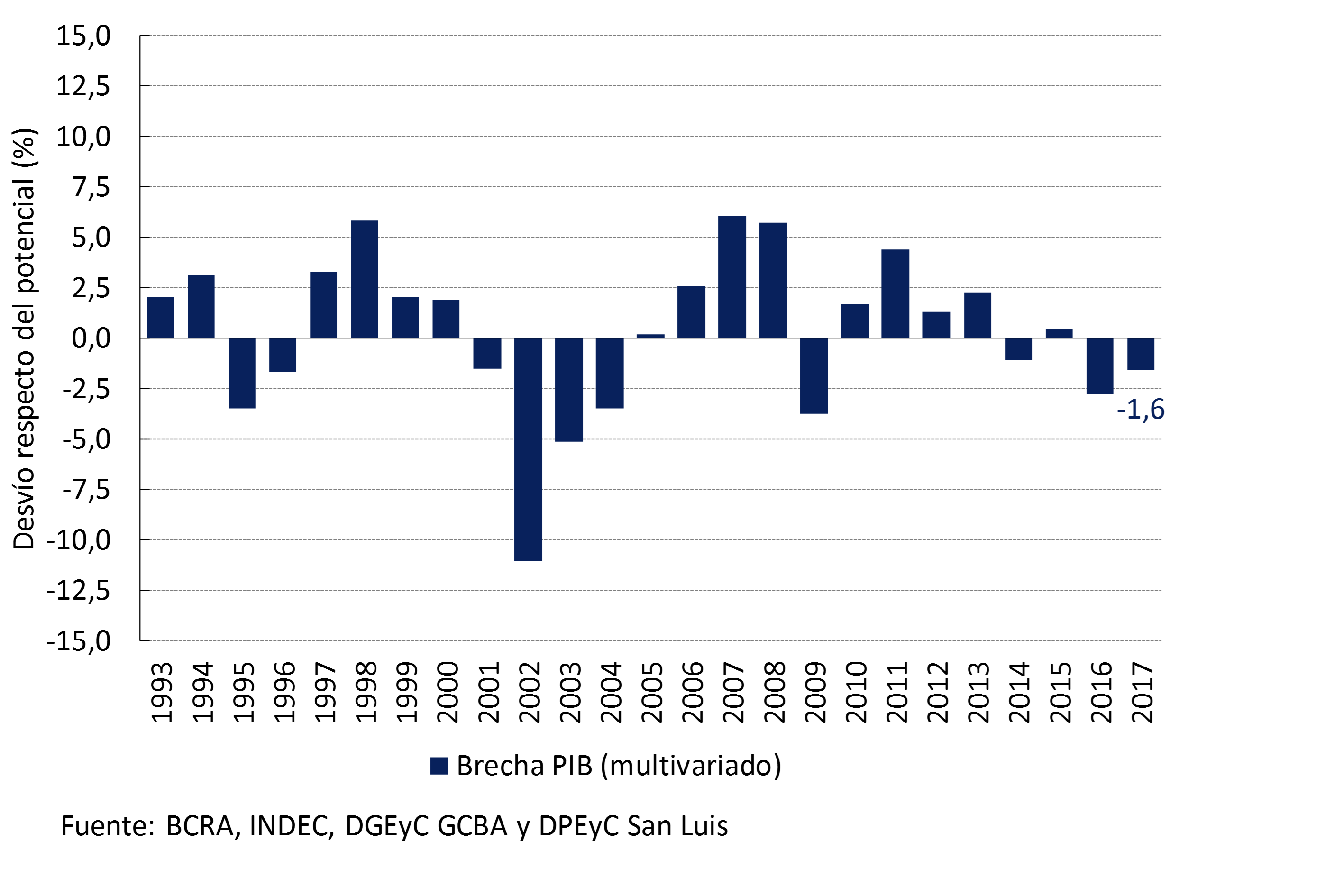
Graph 1 shows the output gap, understood as the deviation of output from its potential, as a percentage. It is possible to distinguish several differentiated periods, in which the output gap alternates its sign. The period 1999-2002, marked by the economic crisis, ended with a pronounced negative output gap. Since 2003, the economy has begun a process of recovery and growth36. In this respect, the output gap was positive again in 2005. This sign will be held until 2015, with the exception of 2009 and 2014. In both years, it becomes negative due to a double effect of positive potential growth and a fall in GDP (this depression is linked in the first case to the effects of the international financial crisis; while in 2014 it is related, among other factors, to the depreciation of January of that year). At the end of the sample, a negative output gap was observed in 2016 (-2.8%), which tended to close in 2017 with a value of -1.6%.
Graph 2 | GDP and potential GDP
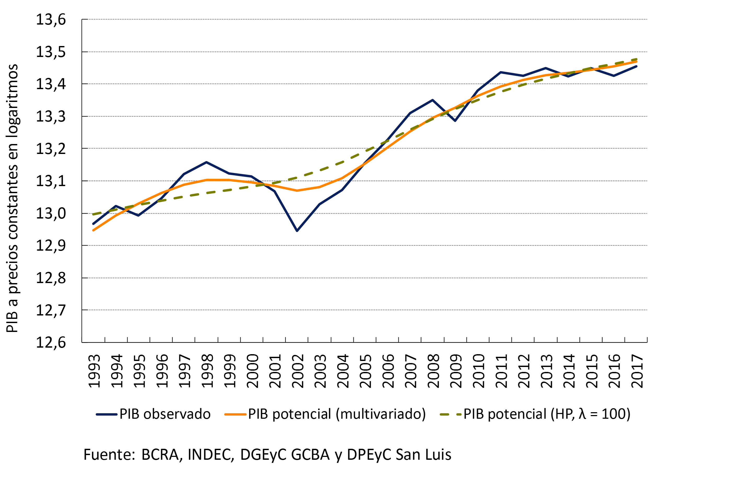
Graph 2 shows the GDP and potential output estimated from the proposed methodology. To have a reference with respect to this last variable, the calculation made from the HP37 filter is incorporated. It is observed that at the end of the interval, the series are similar. Meanwhile, the main differences occur in the 1996-2005 interval, where the multivariate filter captures the short-term evolution of GDP in constant currency more closely. For this reason, the gaps are smaller in absolute value compared to the calculation using the HP filter.
References
Albagli, E. Naudon, A. (2015). What Do We Talk About When We Talk About Potential Product? Mimeo Central Bank of Chile.
Benes, J., Clinton, K., García-Saltos, R., Johnson, M., Laxton, D., Manchev, P., Mathenson, T. (2010). Estimating Potential Output with a Multivariate Filter. IMF Working Paper WP 10/285.
Borio, C., Disyatat, P., Juselius, M. (2013). Rethinking Potential Output: Embedding Information about the Financial Cycle. BIS Working Papers No. 404.
Ljung, L. (1999). System Identification: Theory for the User (2nd ed.). Upper Saddle River. New Jersey: Prentice Hall.
Melolinna, M. Tóth, M. (2016). Output Gaps, Inflation and Financial Cycles in the United Kingdom. Bank of England Staff Working Paper No. 585.
Section 3 / How much does public transport increase?
The Ministry of Transport of the Nation has decided that as of February 1 of this year, new fare schedules will come into force for public passenger transport in the Metropolitan Area of Buenos Aires (AMBA). The tables that will come into force in April and June were also announced. Along with the announcement of the increases, the “SUBE Network” was launched, a system that integrates all modes of public transport in the AMBA (buses, trains and subways) to be able to offer discounts to those who make one or more combinations.
With the entry into force of the “SUBE Network”, the first means of transport taken by the passenger will be paid at full value. The second means of transport used in a period of less than two hours will have a 50% discount, while the third will only pay 25% of the value of the ticket. The proposed increase for February in the value of the full ticket for trains and buses is approximately 33%. In the brackets in which the 50% (25%) discount applies, the rate paid will be reduced by 33% (66%) with respect to the values prior to the increase. The value of the subway ticket remains unchanged on February38 for those who pay full price and is reduced by 50% and 75% for discounted fares.
To estimate the impact on the index of these means of transport on the CPI in February, it is necessary to have the proportion of tickets that will pay the full price and with each discount. For these purposes, we will make three cases of proportionality. Depending on the distribution assumption used, the increases of trains and buses would be between 0% and 15%, while the price of the subway would be reduced between 14% and 25%.
Table 1 | Impact of the increase in the cost of transport on the price index in February
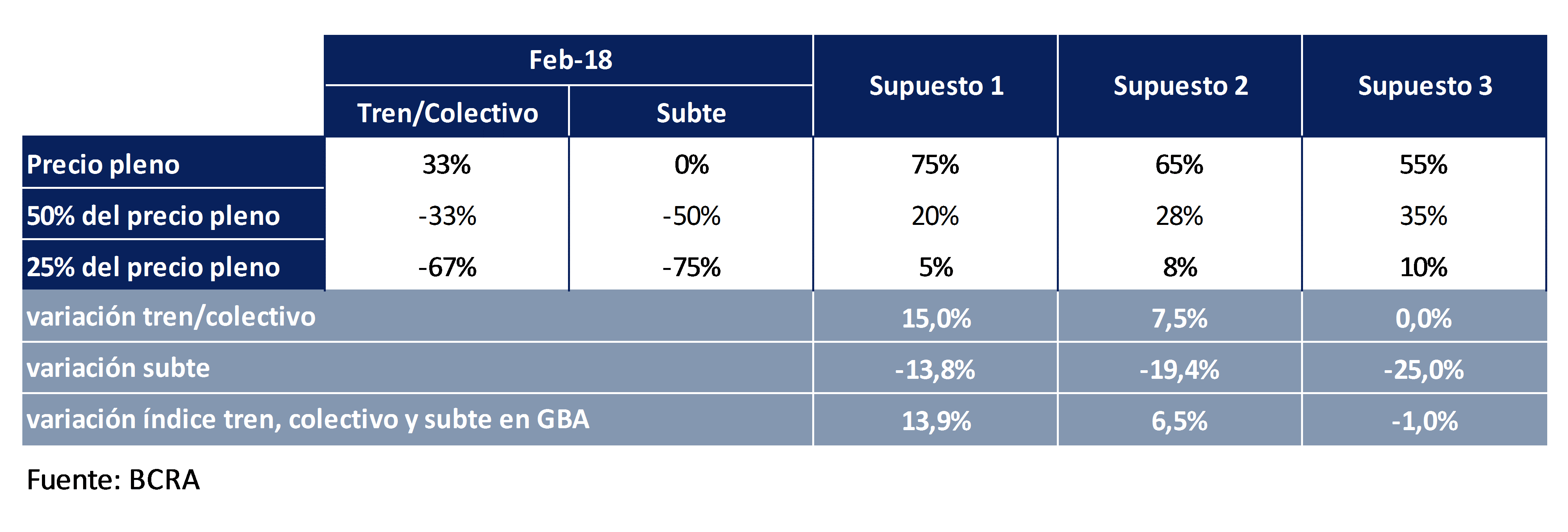
To estimate the effect on the GBA CPI, assuming that INDEC considers these discounts, it is necessary to have the weights of each of these means of transport in the index. The methodology of the current GBA CPI publishes the weighting of public transport, which is 2.8%, but not the breakdown of its components (bus, train, subway and taxi). To estimate the weighting of each of these components, the relative participation they had in public passenger transport of the GBA base 2008 CPI was considered. According to this publication, the bus represented 67% of the aggregate, while the train accounted for 8%, the subway 3% and the taxi the remaining 22%. Using the information described above and the current weighting of public passenger transport, the weighting in the GBA CPI would be: 1.9% for buses, 0.2% for trains, 0.1% for subway and 0.6% for taxi.
Based on these weights, the GBA’s public transport index (excluding taxi) would register a variation in February that could be between -1% and 14%, depending on the assumption made. If we consider that the weighting of the GBA in the national index is close to 50%, the variation of this component in the national index would be practically halved, with an incidence that could vary between 0 and 0.2 p.p.
Section 4 / Pass-through from exchange rate to prices: international evidence
The relationship between changes in the nominal exchange rate and the evolution of domestic prices is of great relevance for monetary policy. Usually, this relationship is studied through pass-through coefficients, which estimate the reaction of the price level to variations in the nominal exchange rate. Conceptually, these coefficients vary according to the underlying cause of the initial movement in the exchange rate. For example, nominal shocks are associated with a higher pass-through of the exchange rate to prices, while real shocks, such as changes in the terms of trade, demand, etc., are associated with lower pass-through ratios. Thus, it is to be expected that in inflationary economies with a preponderance of nominal shocks, the pass-through will be greater than in inflation-targeting economies. This section assesses the international evidence on how the adoption of inflation targeting regimes affected the pass-through of exchange rates to prices, distinguishing between nominal and real shocks. The objective is to try to understand what is to be expected for the relationship between exchange rate and prices in Argentina when low and stable inflation is consolidated, under an inflation targeting scheme.
The sample considered includes five emerging countries that adopted the inflation targeting regime after a prolonged period of moderate/high inflation. The following table presents the periods considered for each economy39 and the average year-on-year inflation in each of them.
Table 1 | Average inflation before and after the adoption of the inflation targeting regime
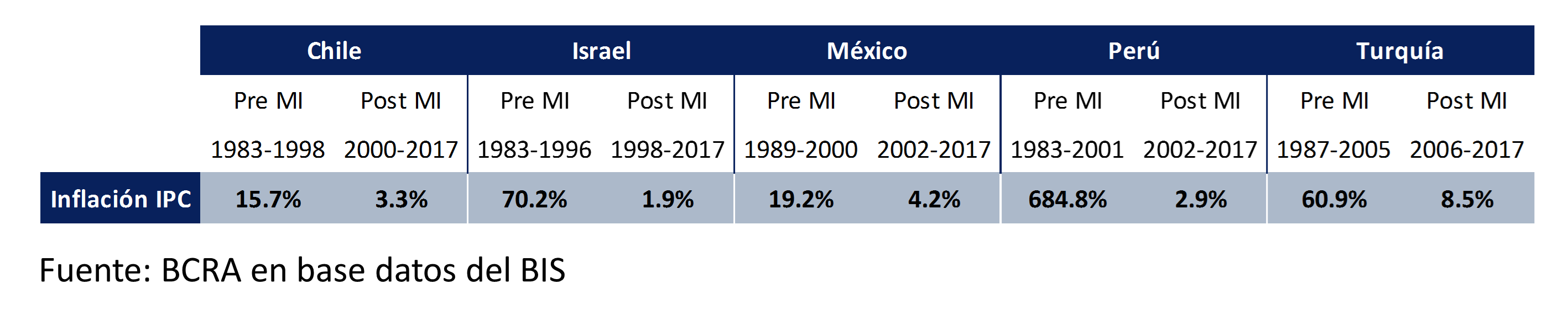
From an autoregressive vector model, the reaction of inflation to a nominal exchange rate shock can be estimated. Figure 1 shows the fraction of exchange rate innovations that are passed on to prices, and the time it takes to do so, before and after the adoption of the inflation targeting regime. In Israel, for example, before the adoption of inflation targets, the immediate reaction of prices to a currency depreciation was 64% on the spot and over time it reached 86%. After the adoption of the inflation targeting regime, these figures fell to an immediate effect of 10% and a long-term effect of 19%. The same pattern is observed for all countries in the sample.
Graph 1 | Unconditional pass-through of nominal exchange rate to CPI prices
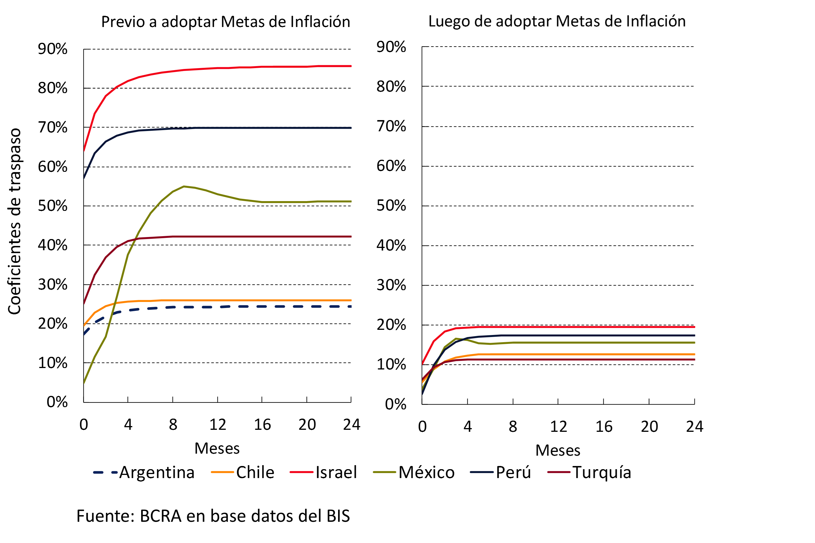
A central aspect of the aforementioned monetary regime is that it proposes to achieve low and stable inflation without using the exchange rate as a nominal anchor. By announcing inflation targets and a set of measures aimed at meeting these targets, central banks are able to get the private sector to anchor its inflationary expectations and to keep the nominal exchange rate floating in line with the demand and supply conditions prevailing in the economy. Together, these two aspects drive a decoupling between the nominal exchange rate and the level of domestic prices, therefore, a reduction in the pass-through coefficients of variations in the exchange rate to domestic prices.
To understand the reasons behind this decrease in pass-through, as initially indicated, it is necessary to consider the primary causes of changes in the exchange rate. In particular, if different determinants generate different exchange rate and price dynamics, the pass-throughs associated with these impulses will be different. It is evident, therefore, that the pass-through of the exchange rate to prices must be studied as a phenomenon conditional on the cause behind the exchange rate movement.
While there are a multitude of determinants of the exchange rate, a simple but intuitive way to group them is by distinguishing between real and nominal factors. Through a structural auto-regressive vector model that includes the real and nominal exchange rates, real and nominal determinants can be discriminated, identifying the latter as those that do not affect the real exchange rate in the long run40. In this way, impulse-response functions are obtained for each type of impulse, from which the conditional transfers in each of them are computed. Figure 2 shows the pass-through coefficients that elicit both real and nominal impulses, distinguishing between the stages before and after the introduction of inflation targeting.
Graph 2 | Conditional transfer of nominal exchange rate to CPI prices
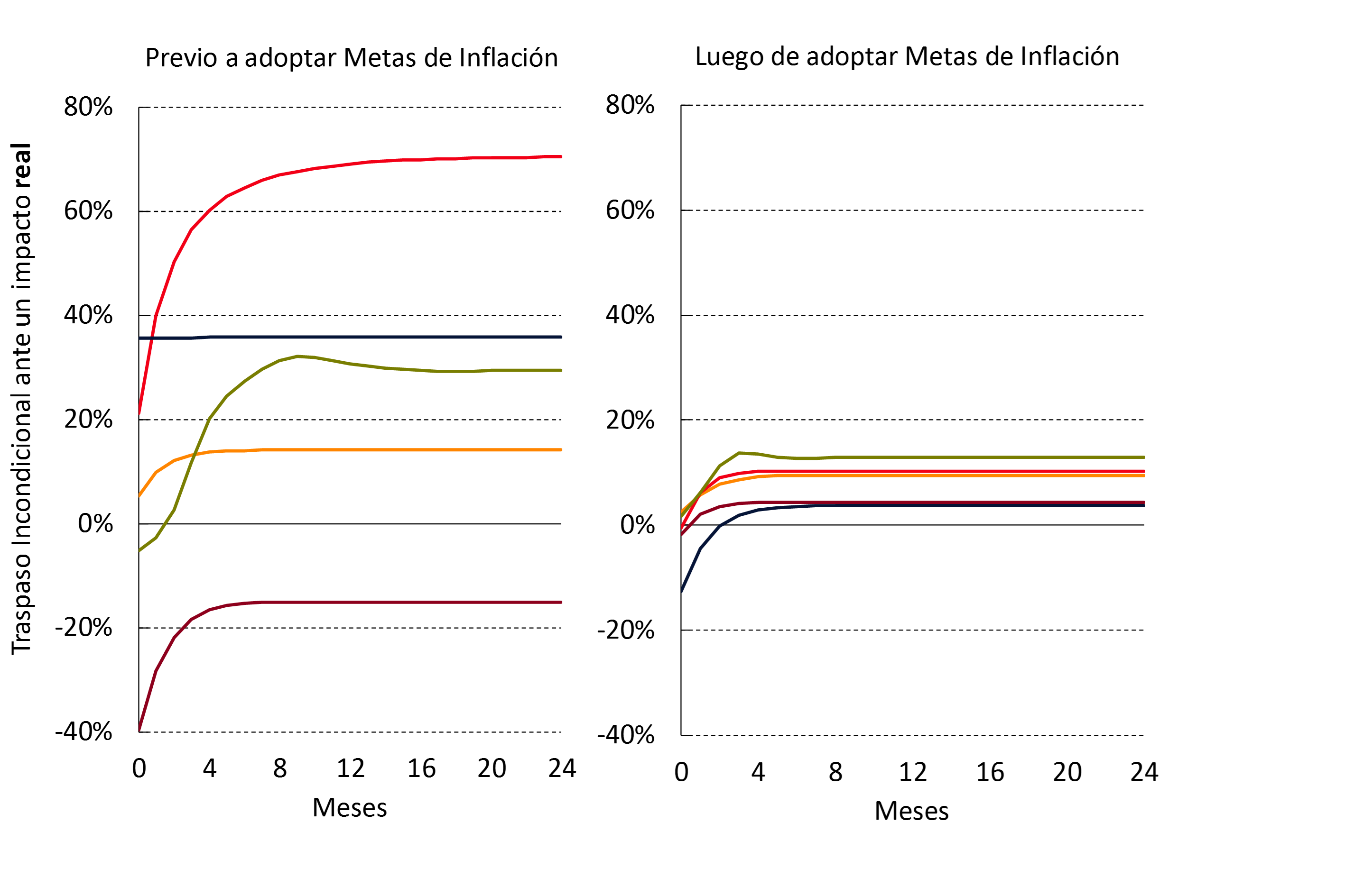
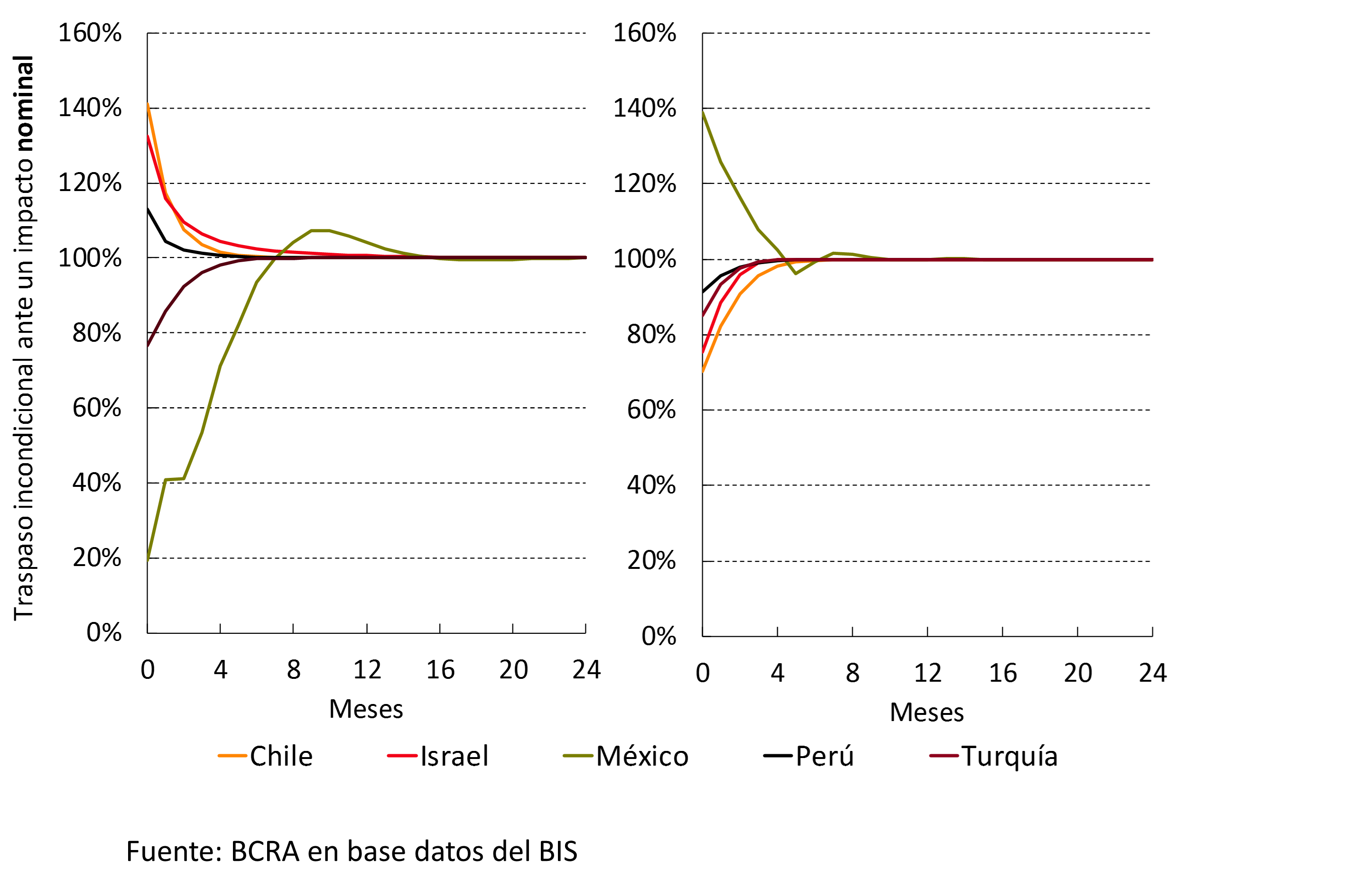
Two empirical regularities of interest shown in Figure 2 are (a) the fact that the pass-through to inflation of depreciations caused by a real shock is lower than that caused by a nominal shock and (b) that the pass-through to prices of both types of shocks tends to be lower under inflation targeting. It is important to note that negative pass-through values in the face of real shocks are to be expected under managed exchange rate schemes. This is because negative real shocks require real depreciations to accommodate the shock. If the nominal exchange rate does not depreciate sufficiently because it is managed, the real devaluation will occur due to falls in prices, thus explaining a negative pass-through. 41 Extreme examples of these situations are Argentina after the devaluation of Brazil, or Greece during the European crisis in 2010.
Another empirical regularity is that under inflation targeting, nominal shocks are much less important. In fact, the percentage of nominal exchange rate volatility attributed to nominal shocks decreases, after the adoption of inflation targets, from 17 to 3% for Chile, from 60 to 8% in Israel, from 25 to 5% for Mexico, from 73 to 14% for Peru, and from 45 to 6% for Turkey. This is by virtue of a monetary policy focused on reducing the volatility of inflation around the target.
Thus, these results allow us to understand why the pass-through of depreciation to inflation is lower under inflation targeting: on the one hand, the impact of each shock is smaller and, on the other, in the inflation targeting regime, nominal shocks are much less important.
What are the implications of this analysis for Argentina? Unfortunately, the sample for Argentina in the inflation targeting period is too short to replicate this same exercise. We can compute the transfer for Argentina in the period from 2007 to 2015, which is included in the left panel of Graph 1. As can be seen, the pass-through in that period is comparable to that of Chile, and somewhat lower than that of Turkey, before the adoption of the inflation targets. Given the experience of these countries, where the pass-through was reduced by about half with the new monetary policy scheme, the outlook for the Argentine case points to a significant reduction in the pass-through of exchange rate movements to prices.
Section 5 / The sustainability of LEBACs
When studying the evolution of an institution’s liabilities and their eventual sustainability, it is essential to take into account three fundamental variables: the evolution of assets, the evolution of revenues and the future income outlook of the institution.
In the last two years, the Central Bank has acquired foreign currency with the aim of reaching a level of international reserves similar to that of other countries in the region that operate under an inflation targeting scheme and a floating exchange rate (see Section 5.4). The Central Bank has accompanied the purchases of foreign assets carried out with sterilization operations, so as not to generate an excess supply of money that places the interest rate outside the level established to achieve the inflation target. These sterilization operations consist of the sale of LEBAC by the Central Bank or the realization of passive passes by financial institutions, both aimed at absorbing monetary base. As a result, foreign assets have been increasing along with the non-monetary liabilities of the Central Bank (LEBAC and net passes).
The ratio of LEBAC plus net passes to international reserves has remained broadly stable since the end of 2015, while it had risen significantly between 2011 and 2015 as a result of falling reserves. When discounting the swap with China from international reserves, it can be seen that the increase between 2011 and 2015 is more pronounced and that stability since 2015 is transformed into a significant fall in LEBACs plus net passes in relation to foreign assets (see Chart 1).
Graph 1 | Ratio of LEBAC and net passes to international reserves (December average)
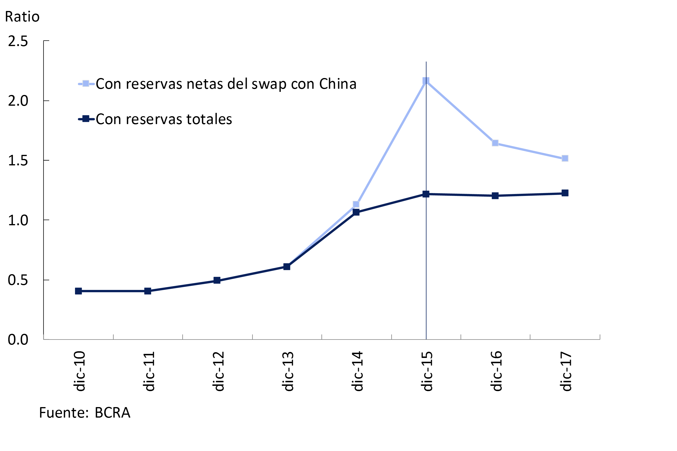
After considering the evolution of the asset in the analysis, the evolution of GDP is incorporated. Using ratios in terms of GDP is the usual way of analysing the evolution of macroeconomic variables over time to discount the evolution that accompanies the growth of the real economy and inflation. It also makes sense because the Central Bank’s revenues are associated with both variables.
The stock of non-monetary liabilities, discounting the reserves acquired since March 201642, fell from 7.2% of GDP in March 2016 to 6.2% of GDP at the end of 2017 (see Chart 2). It is true that this stock grows when the acquired reserves are not discounted, but it has already been seen that the correct thing to do is to analyse the evolution of the liabilities and the assets generated by them together.
Graph 2 | LEBAC plus net passes minus Acquired International Reserves
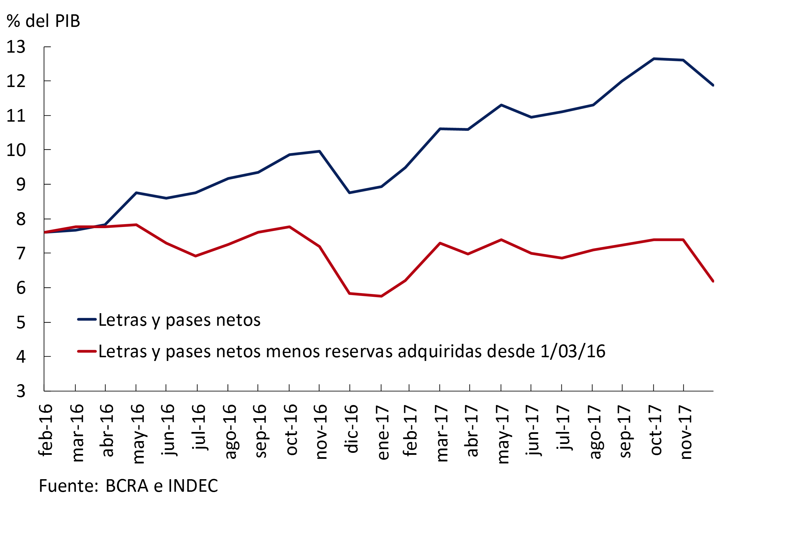
Finally, it remains to analyze the future revenues of the Central Bank, which constitute an economic asset not accounted for in its balance sheet. The Central Bank receives revenue, called seigniorage, for issuing a liability (monetary base) that does not pay an interest rate (and with a small marginal cost of issuance) but that is demanded by economic agents to use it as a means of payment and store of value. 43 When making transfers to the National Treasury, the monetary authority shares a portion of that seigniorage. Through a series of assumptions about the evolution of the economy, an estimate of future seigniorage revenues is made. And based on the agreement with the Treasury on transfers (see Figure 5.8), it is possible to assess how much of this income will remain in the Central Bank and what the impact will be on its economic balance sheet.
Considering a scenario in which the economy grows at 3% per year, with inflation of 5% per year and with the monetary base stable at 9.8% of GDP (level of December last year), the Central Bank would obtain an annual seigniorage of 0.74% of GDP. If transfers to the Treasury for 0.3% of GDP are subtracted from this flow, according to the agreement reached, and the general and printing expenses of the Central Bank for 0.08% of GDP, and this net income is considered as a perpetuity, the present value of net seigniorage stands at 37% of GDP. 44 In this scenario, this source of funds is three times the magnitude of the non-monetary liabilities that the monetary authority currently has, at around 12% of GDP. Even if illiquid instruments, such as non-transferable bills and the stock of transitory advances to the Treasury, are not considered in assets, economic net worth remains at high levels (34.7% of GDP) (see the following table, which compares the balance sheet at the end of 2017 with the “economic” balance sheet that considers the present value of seigniorage in assets).
Table 1 | Comparison of the “accounting” balance sheet at the end of 2017 with the “economic” balance sheet
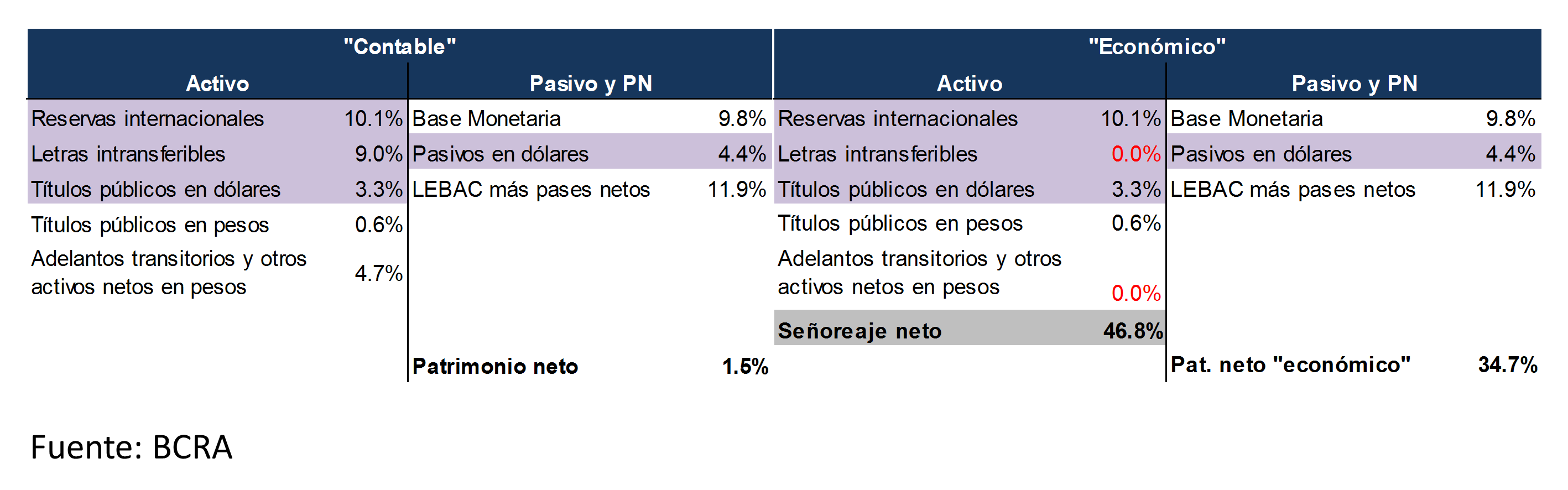
In conclusion, when we take into account the acquisition of foreign assets that was financed with monetary liabilities, the evolution of GDP and the projection of future revenues of the Central Bank, we see that: non-monetary liabilities net of acquired reserves have fallen as a percentage of GDP; and that, even without discounting these foreign assets, future revenues are more than enough to meet them.
References
1 See Brazil and its Effect on Argentine Activity: A Look at the Commercial Channel, in Ideas de Peso. As indicated therein, this estimate is among the most cautious, with others foreseeing a greater impact.
2 U.S. growth in 2018 could be boosted by the fiscal stimulus resulting from the recently approved tax reform.
3 For more details, see the corresponding Fed document published on its website.
4 A fall in the terms of trade has an unfavorable impact on Argentina’s trade balance, and an increase has a favorable impact.
5 REM of November 2017.
6 This decrease in the ILA in December is insufficient to indicate a change in the phase of economic activity since only one of the three signals required to issue a pivot point alert was met. Note that in other months corresponding to periods of expansion, such as September/October 2016, similar falls in the ILA have been evidenced without a change of phase in the economic cycle. For more details, see Section 3 / BCRA’s Leader Index of Economic Activity, IPOM, January 2017.
7 Other construction and other fixed assets grew 0.8% YoY and 3.7% YoY, respectively.
8 The quarterly variations of the IBIF-BCRA indicator are a weighted average of the seasonally adjusted quarterly variations of the ISAC (INDEC), imports of capital goods (INDEC) and national production of capital goods (FIEL). The weights correspond to the weight of construction, investment in imported durable production equipment (EDP) and national EDP in the IBIF of the previous quarter. The groupings “Other constructions” and “Other fixed assets” that are part of the IBIF are not considered in the indicator due to the lack of leading indicators for these concepts. With data as of November, the ISAC rose 3.7% s.e. quarterly, imports of capital goods fell 1.3% s.e. while the national production of capital goods rose 0.6% s.e.
9 The estimation of the trend-cycle of a series is very sensitive to the last data used, which is why it can be inferred that the growth of the trend in private consumption for the third quarter of 2017 would have been higher if the improvement of the original series in the fourth quarter had been confirmed.
10 For more details see Section 1/ Private consumption, a variable difficult to follow in real time, IPOM July 2017.
11 For more details, see the Financial Stability Report for the second half of 2017.
12 The lending and passive rates set by financial institutions were released. The possible uses of the loanable capacity available in foreign currency were expanded, avoiding currency mismatches in balance sheets.
13 As of October 2017, 73.4% of registered employment was employed in the private sector of the economy, 0.2 p.p. above December 2016.
14 According to INDEC, the Gini coefficient of people’s per capita family income in urban agglomerations fell from 0.451 to 0.427 between the third quarter of 2016 and the third quarter of 2017.
15 According to data from the Ministry of Labor, Employment and Social Security corresponding to the Argentine Integrated Pension System (SIPA), deflated by National CPI.
16 The Argentine tax system is characterized by the existence of strongly distorting taxes such as the Tax on Bank Debits and Credits, Gross Income and Export Duties.
17 The series of CPIs of the INDEC of national coverage as of Dec-16 is considered, spliced with the CPI NP calculated by the BCRA based on the CPIs of the City of Buenos Aires, Córdoba and San Luis.
18 GBA CPI prepared by INDEC since April 2016 spliced with the CPI of the City of Buenos Aires.
19 For the impact on the expenses of the increase in electricity and gas services.
20 To analyze the behavior of core inflation by goods and services, the CPI of the City of Buenos Aires will be used, since there is not enough disaggregated information available to carry out this analysis on the CPI prepared by INDEC. The dynamics of the prices of goods and services in both indicators are similar, both at the monthly level and in the annual accumulated variation.
21 The basket of the wholesale price index at market prices (IPIM) is mainly composed of goods.
22 These results correspond to the survey carried out between December 22 and 9 a.m. on December 28, 2017, prior to the announcement of the modification of the inflation targets.
23 An indicator closely monitored by the Central Bank to identify price dynamics is the three-month moving average of core inflation. Core inflation is taken to reduce the impact of changes in regulated prices, which are not affected by monetary policy and are especially important in a period of reversal of tariff arrears, and the three-month average is taken to reduce the volatility inherent in any monthly indicator of price variation.
24 See the IPOM of October 2017, Section 1 / Exchange rate float and current account volatility.
25 See communication “A” 6426 of January 10, 2018.
26 The real interest rate was calculated with the three-month average of the expected monthly general inflation of the Market Expectations Survey carried out by the Central Bank. The use of the three-month average makes it possible to soften the transitory impacts on the inflation rate.
27 The Argentine tax system is characterized by the existence of highly distorting taxes such as the Tax on Bank Debits and Credits, Gross Income and Export Duties.
28 The national and provincial governments signed the so-called Fiscal Consensus. Law 27.429.
29 The Gross Income Tax is a provincial tax that is applied as a percentage of the turnover of firms. Each jurisdiction uses its own individual rates and parameters to decide whether or not a type of company should pay. It is considered a highly distorting tax since an aliquot is applied to the turnover regardless of its profits. Unlike VAT, a good that goes through different stages of production can be affected by the gross income tax in each of them, accumulating this burden, which deepens its distorting nature.
30 Australia is an example of an economy that has shown sustained growth in per capita income and has managed to become considered an advanced country. In his case, the process of structural reform lasted at least three decades between the 1970s and 1990s (Banks, 2005: Structural Reform Australian-style: Lessons for Others?)
31 There are, however, other views on the potential product. In neo-Keynesian models, it is usually defined as that level associated with purely flexible prices and wages, that is, without nominal rigidities. On the other hand, even in an environment of low and stable inflation, output could be on an unsustainable path, due to the presence of financial imbalances. For this reason, and especially since the 2008 international crisis, institutions in countries with significant financial depth have developed “financially neutral” potential output calculations that include financial condition indices (Borio et al., 2013; Melolinna Tóth, 2016).
32 Among the countries whose central banks use or have used this technique are Brazil, Canada, Chile, Colombia, the United Kingdom, New Zealand and Peru. In addition, the European Central Bank and international organizations such as the IMF and BIS make estimates under this methodology.
33 In particular, the method of maximum regularised likelihood was used. For more information, see Ljung, L. (1999).
34 In addition, the model incorporates steady-state conditions in terms of economic growth and unemployment, assumptions that were completed from the historical average of the series since 2004.
35 Non-Accelerating Inflation Rate of Unemployment.
36 The unemployment gap evolves in a similar way, in terms of the signs and trends that occur each year, to the output gap in the period 1993-2004. During the period 2005-2015, the variable does not present a negative value in any year (while the output gap has it in 2009 and 2014). Meanwhile, the final biennium again presents a negative gap (-1.1% in 2016 and -1.5% in 2017).
37According to certain standard techniques for annual frequencies, a smoothing parameter of λ=100 was chosen.
38 The increase is scheduled for April and June.
39 The dates of adoption of the inflation targeting regime were taken from Hammond, Gill (2012). “State of the art inflation targeting”, Bank of England.
40 For more detail on this methodology, see Enders and Lee, 1997, “Accounting for real and nominal exchange rate movements in the post-Bretton Woods period,” Journal of International Money and Finance.
41 These negative real shocks have more negative consequences for activity and employment when the nominal exchange rate cannot be adjusted appropriately. See, for example, Schimtt-Grohe and Uribe, 2016, “Downward Nominal Wage Rigidity, Currency Pegs, and Involuntary Unemployment,” Journal of Political Economy.
42 The total international reserves are not taken into account, but only those acquired since March 2016, because the focus is on the result of the policy of implementing monetary policy with interest rates, exchange rate floats and occasional sterilized operations carried out since then.
43 This income can be broken down into two factors: (1) the public’s desire to modify its demand for money (from its real balances), which depends on the interest rate and the level of economic activity; and 2) the inflationary tax, that is, the loss of purchasing power by holding money due to the effect of inflation, which represents a transfer of resources from the public to the treasury. Although the inflationary tax is not desirable from a distributional point of view, the target inflation rate from 2020 onwards is at the levels shown by the economies of the region or other emerging economies, and is associated with the achievement of price stability.
44 The present value of seigniorage with the variables in long-run values can be expressed as follows:
VPS=frac{Delta BM}{PIB} (frac{1+g}{r-g})
Where,frac{Delta BM_t}{PIB_t}= frac{(BM_t-BM_{t-1} )} {PIB_t} is the annual seigniorage in terms of GDP (0.74% of GDP for all periods minus 0.3% of GDP from transfers minus 0.08% of primary expenditures of the Central Bank), r is the real interest rate (4%), and g is the growth rate of the economy (3%). The present value of seigniorage can also be expressed by considering the present value of the interest not paid for using a monetary liability minus the initial stock of the monetary base:
VPS=i frac {bm} {(1+i)} (frac {1+r}{r-g})-bm
In this case, the result would be: 86.0% (corresponding to the present value of the unpaid interest on the monetary base) minus the present value of transfers and primary expenditures in terms of GDP (30.9% and 8.2%, respectively), which gives 46.8% of GDP. If 9.8% of the monetary base stock is subtracted from this value, we arrive at 37% of the GDP obtained with the previous formula. This is the way in which seigniorage is expressed in the balance sheet in Table I. For a detailed analysis of the calculation of government seigniorage, see Buiter, W. (2007): “Seigniorage”, NBER, working paper No. 12919.
Glossary of abbreviations and acronyms
€: Euro
Acum.: Cumulative
AFCP: Portland Cement Manufacturers Association
AFIP: Federal Administration of Public Revenues
AUH: Universal Child Allowance for Social Protection
BADLAR: Buenos Aires Deposits of Large Amount Rate (interest rate paid for fixed-term deposits of more than one million pesos in the 30 to 35-day bracket by the average of banking entities)
BCB: Central Bank of Brazil
BCBA: Buenos Aires Stock Exchange
ECB: European Central Bank
BCRA: Central Bank of the Argentine Republic
BONAR: Argentine Nation Bond
CABA: Autonomous City of Buenos Aires
CEMBI+: Corporate Emerging Market Bond Index Plus
CEMBI+AR: Corporate Emerging Market Bond Index Plus Argentina
ECLAC: Economic Commission for Latin America and the Caribbean
CER: Reference Stabilization Coefficient
FIGURE: Research and Training Center of the Argentine Republic – Central de Trabajadores de la Argentina (CTA)
COICOP: Classification of Individual Consumption According to Purpose
CNV: National Securities Commission
Contrib.: Contribution
S Fuels Energy
DJVE: Affidavits of Foreign Sales
e: Dear
EDP: Durable Production Equipment
EIL: Survey of Labor Indicators
EMAE: Monthly Estimator of Economic Activity
EMBI+: Emerging Markets Bond Index Plus
EMBI+AR: Emerging Markets Bond Index Plus Argentina
EMBIG: Emerging Market Bond Index Global
ENGHo: National Survey of Household Expenditure and Income
EPH: Permanent Household Survey
excl.: Excluding
Fed: Federal Reserve of the United States
FIEL: Latin American Economic Research Foundation
IMF: International Monetary Fund
IMF WEO: World Economic Outlook
FOB: Free on Board (purchase and sale operations carried out by boat)
FOMC: Federal Open Market Committee
GBA: Greater Buenos Aires
A.I.: Year-on-year
IAMC: Argentine Institute of Capital Markets
IBIF: Gross Domestic Fixed Investment
ICC: Consumer Confidence Index prepared by the Torcuato Di Tella University
ICC-INDEC: Construction Cost Index
IGA-OJF: Orlando J. Ferreres General Activity Index
ILA: Activity Leader Index
ILCO: BCRA’s Leading Indicator of Private Consumption
INDEC: National Institute of Statistics and Censuses
INML: Liniers Market Steer Index
CPI: Consumer Price Index of national coverage released by INDEC
IPCBA: Consumer Price Index of the City of Buenos Aires
CPI Cordoba: Consumer Price Index of the Province of Cordoba
CPI GBA: Consumer Price Index of Greater Buenos Aires
CPI-NP: Weighted National Indicator
San Luis CPI: Consumer Price Index for the Province of San Luis
IPIB: Basic Domestic Price Index
IPIM: Internal Wholesale Price Index
MPPI: Commodity Price Index
IPOM: Monetary Policy Report
ITCNM: Multilateral Nominal Exchange Rate Index
ITCRM: Multilateral Real Exchange Rate Index
VAT: Value Added Tax
kg: Kg
LAC: Latin American Consensus Forecasts
LEBAC: Central Bank Bills (Argentina)
LELIQ: Central Bank Liquidity Bills (Argentina)
LFPIF: Financing Line for Production and Financial Inclusion
M2: Banknotes and coins + quasi-currencies in circulation + current accounts in $ and savings accounts in $
Mens.: monthly
MERVAL: Buenos Aires Stock Exchange
mill.: Million
Min.: Ministry
IPM: Input-output matrix
MOA: Manufactures of Agricultural Origin
MOI: Manufactures of Industrial Origin
MRO: Main refinancing operations
MSCI: Morgan Stanley Capital International Index
MULC: Single and Free Exchange Market
NEA: Northeast Argentina
NG: General level
NOA: Northwest Argentina
OECD: Organisation for Economic Co-operation and Development
OPEC: Petroleum Exporting Countries
bp: Basic points
p.p.: Percentage points
p: Projected
PAMI: Social Work for Retirees and Pensioners
PCE: Personal consumption expenditures
PCP-BCRA: Contemporary BCRA GDP Prediction
EAP: Economically Active Population
GDP: Gross Domestic Product
PMI: Purchasing Managers’ Index
PP: Primary Products
Prom. Moving Average: Moving Average
Avg.: Average
R$: Real
REM: BCRA Market Expectations Survey
REPO: Repurchase Agreement (Operación de Recompra)
ROE: Records of Export Operations
REPO Round: Average interest rate of 1-business day transactions between financial institutions in the guaranteed market
S.A: Sociedad Anónima
s.e.: Series without seasonality
SSPM: Private Consumption Indicator prepared by the Ministry of Finance
TFF: Federal Funds Rate
tonnes: tonnes
TN: National Treasury
APR: Annual Nominal Rate
Trim.: Quarterly / Quarter
ICU: Utilization of installed capacity
US$: US Dollars
UTDT: Universidad Torcuato Di Tella
UVA: Unit of Purchasing Value
Var.: Variation
Vol.: Volume
YPF SA: Yacimientos Petrolíferos Fiscales Sociedad Anónima
Share on


