Summary
As indicated in its Organic Charter, the Central Bank of the Argentine Republic “aims to promote, to the extent of its powers and within the framework of the policies established by the National Government, monetary stability, financial stability, employment and economic development with social equity”.
Without prejudice to the use of other more specific instruments for the fulfillment of the other mandates – such as financial regulation and supervision, exchange rate regulation, and innovation in savings, credit and means of payment instruments – the main contribution that monetary policy can make for the monetary authority to fulfill all its mandates is to focus on price stability.
With low and stable inflation, financial institutions can better estimate their risks, which ensures greater financial stability. With low and stable inflation, producers and employers have more predictability to invent, undertake, produce and hire, which promotes investment and employment. With low and stable inflation, families with lower purchasing power can preserve the value of their income and savings, which makes economic development with social equity possible.
The contribution of low and stable inflation to these objectives is never more evident than when it does not exist: the flight of the local currency can destabilize the financial system and lead to crises, the destruction of the
price system complicates productivity and the generation of genuine employment, the inflationary tax hits the most vulnerable families and leads to redistributions of wealth in favor of the wealthiest. Low and stable inflation prevents all this.
In line with this vision, the BCRA assumes as its primary objective to reduce inflation. As part of this effort, the institution publishes its Monetary Policy Report on a quarterly basis. Its main objectives are to communicate to society how the Central Bank perceives recent inflationary dynamics and how it anticipates the evolution of prices, and to explain in a transparent manner the reasons for its monetary policy decisions.
1. Monetary policy: assessment and outlook
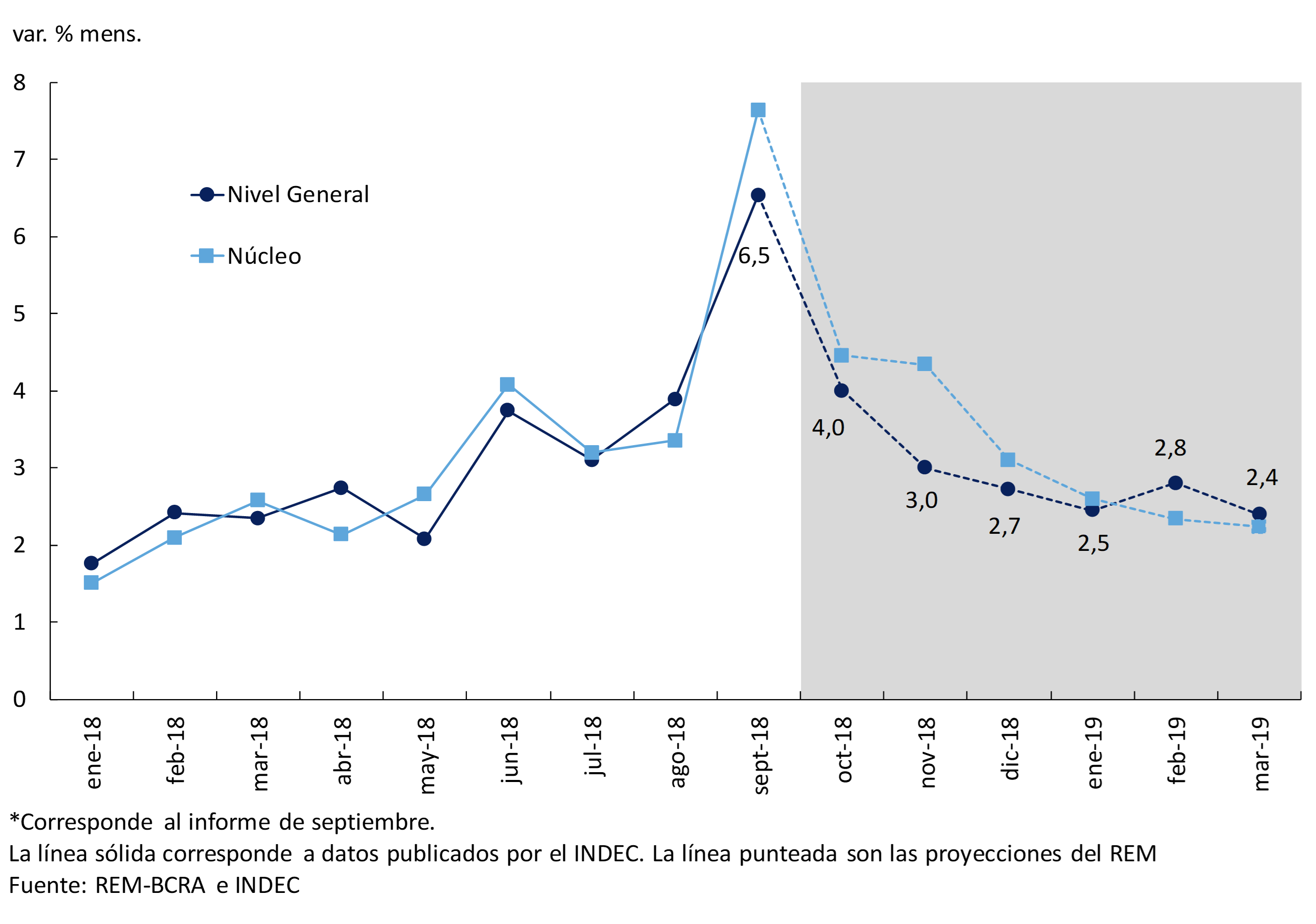
Inflation accelerated sharply in the third quarter of 2018, reaching a monthly average of 4.5% and a record of 6.5% in September. This increase was associated with the depreciation of the peso, which began in April but again marked a high record at the end of August. This second episode of exchange rate instability, in August, deepened uncertainty, led to a further correction in prices and raised the risk of a de-anchoring of inflationary expectations. Analysts’ 12-month inflation expectations went from 24.1% at the end of July to 33.4% at the end of August (average of the Market Expectations Survey).
With the aim of recovering the anchor on expectations and resuming the path of disinflation, the Central Bank of the Argentine Republic (BCRA) modified its monetary policy scheme at the end of September, leaving aside the inflation targeting regime implemented until that moment. It did not yield the expected results. However, target schemes are widely used around the world, both by advanced and emerging economies, and have been successful in ensuring an environment of nominal stability.
The new monetary policy regime that came into effect on October 1 stems from the need to establish a concrete and powerful commitment, immediately observable and verifiable by the public. Thus, the Central Bank undertakes not to increase the monetary base until June 2019. The zero growth of the monetary base constitutes a challenging commitment, since this aggregate had been growing at a rate of more than 2% per month and, given the expected price increases in the coming months, the real monetary base will be decreasing in the new scheme. This monetary aggregate was chosen because it is the one under the direct control of the BCRA. The goal of zero nominal monthly growth of the monetary base will be adjusted with the seasonality of the months of December and June, when the demand for money increases, avoiding an excessive contractionary bias in monetary policy.
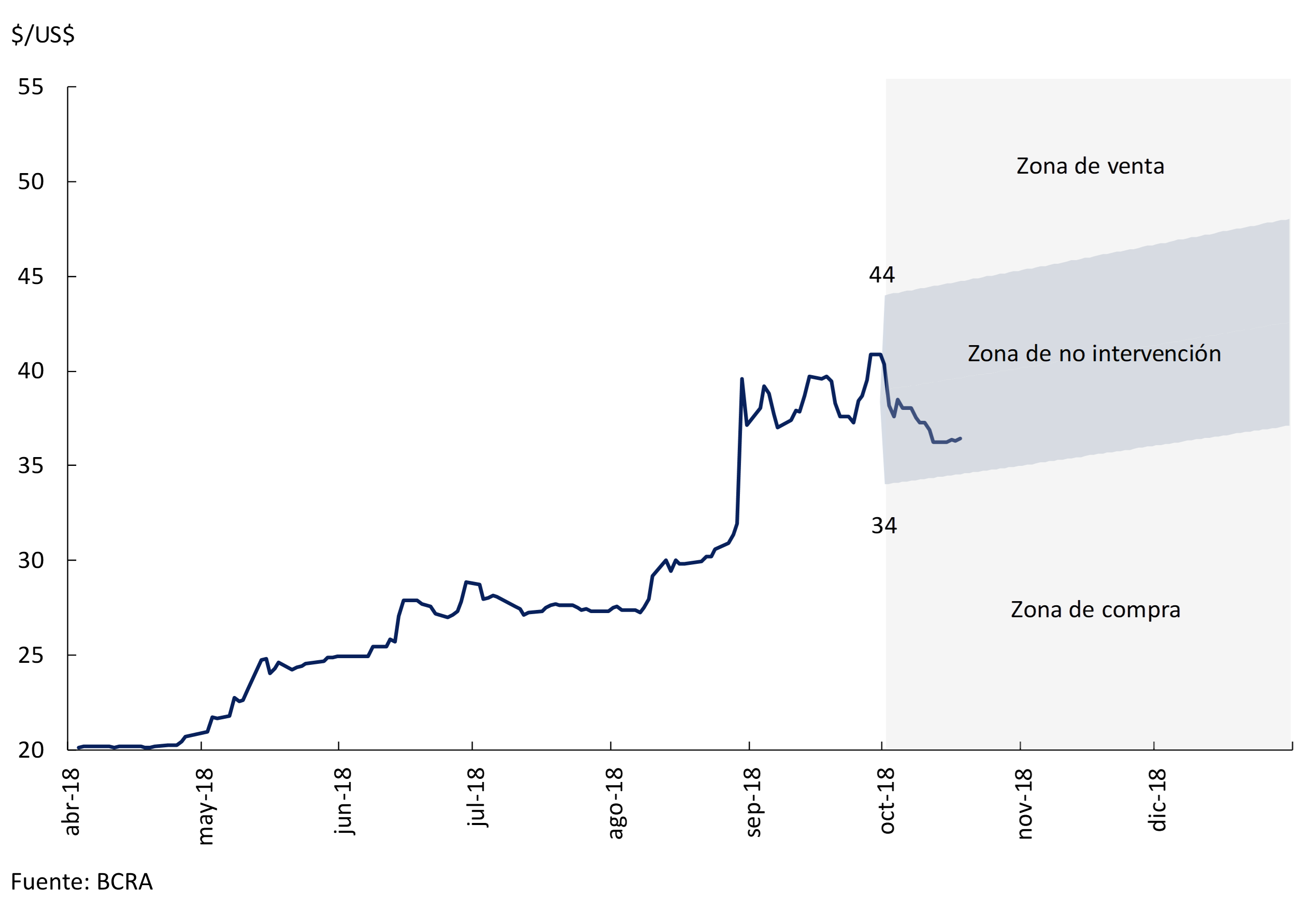
The monetary base objective is complemented by the definition of foreign exchange intervention and non-intervention zones for the exchange rate until the end of 2018. The non-intervention zone was defined on October 1 for an exchange rate of 34 pesos per dollar at the lower limit and 44 pesos per dollar at the upper limit. These limits are adjusted daily at a rate of 3% per month. Above the non-intervention zone, the BCRA can make foreign currency sales of up to 150 million dollars per day, generating an additional monetary contraction at times of greater weakness of the peso. On the other hand, the BCRA can make purchases of foreign currency when the peso appreciates and is below the non-intervention zone. The BCRA may decide whether or not to withdraw the pesos injected by the purchase of foreign currency in the purchase zone, according to the progress of inflation and its expectations. Within the non-intervention zone, the exchange rate fluctuates freely. This system adequately combines the benefits of exchange rate flexibility to face real shocks with the possibility of limiting excessive and disruptive fluctuations that may appear in a still shallow exchange market like ours.
The new monetary policy scheme is also consistent with the primary fiscal balance in 2019 and surplus in 2020 targets established by the Ministry of Finance. The Central Bank does not make any more transfers to the Treasury. The elimination of this source of monetary issuance reinforces the BCRA’s commitment to decreasing inflation over time and ends with a growth factor of the Central Bank Bills (LEBAC) in previous years, and which will not be present in the future in the dynamics of the Liquidity Bills (LELIQ).
The goal of zero growth of the monetary base is established in terms of the monthly average of this variable, so the complete evaluation of its compliance in the first month of validity can be made once October ends. However, to make a preliminary assessment and taking into account the intra-month seasonal behavior of the variable, we can establish a comparison between the average monetary base in the first 21 days of October and its average in the same period of the previous month. We see that the monetary base was reduced by 24.5 billion pesos. This reduction required an additional effort in this period, since in the first two weeks of September the coefficient of unpaid reserve requirements was lower. If the monetary base for September were corrected for this factor, the average for October to the 21st would be 60.5 billion pesos lower than that of the same period in September.
In terms of economic activity, GDP fell by 4% in the second quarter seasonally free of seasonality compared to the previous quarter. The sharp fall in agricultural output as a result of the drought was decisive, but there was also a 1.1% non-seasonal decline in non-agricultural output as a result of the financial and exchange rate tensions that have been evident since April. Both leading indicators and analysts’ perspectives show that the fall in non-agricultural output would continue in the third quarter, as a result of the deepening context of financial uncertainty and the acceleration of inflation.
The BCRA’s view is that the monetary plan for zero growth of the monetary base, together with the announcement of a zero primary fiscal deficit for 2019 made by the Ministry of Finance, is the necessary tool to begin to reduce this uncertainty and reduce both expectations and inflation rates in the coming months. The monetary authority also considers that it is necessary to reduce this uncertainty so that economic activity can begin the path of a recovery on a sustainable basis.
2. International context
Conditions of access to international financial markets in emerging economies continued to deteriorate during the third quarter of the year, although at a slower pace than during the previous quarter. Among the main explanatory factors are the rise in interest rates and the expectation of less monetary stimulus by the Federal Reserve of the United States (Fed), along with new signs of trade tensions between some of the largest economies. All these elements led to an outflow of capital from emerging countries, an increase in sovereign risk premiums, and a depreciation of their currencies. The most affected economies were those with pronounced external imbalances and/or high levels of indebtedness.
During the quarter, a positive performance of world economic activity continued to be observed, including Argentina’s main trading partners. The growth forecast for 2019, pari passu with the projected levels of the real exchange rate, allows us to expect a marked improvement in the performance of the Argentine external sector, with positive impacts on the level of local activity.
Taking into account the deterioration in financial conditions together with the level of activity of trading partners, the international context poses a mixed scenario for Argentina. Even more contractionary international financial conditions, together with a deepening of protectionist measures, continue to be the main risks of the international scenario facing the local economy.
2.1 The level of activity of our business partners improves in 2019
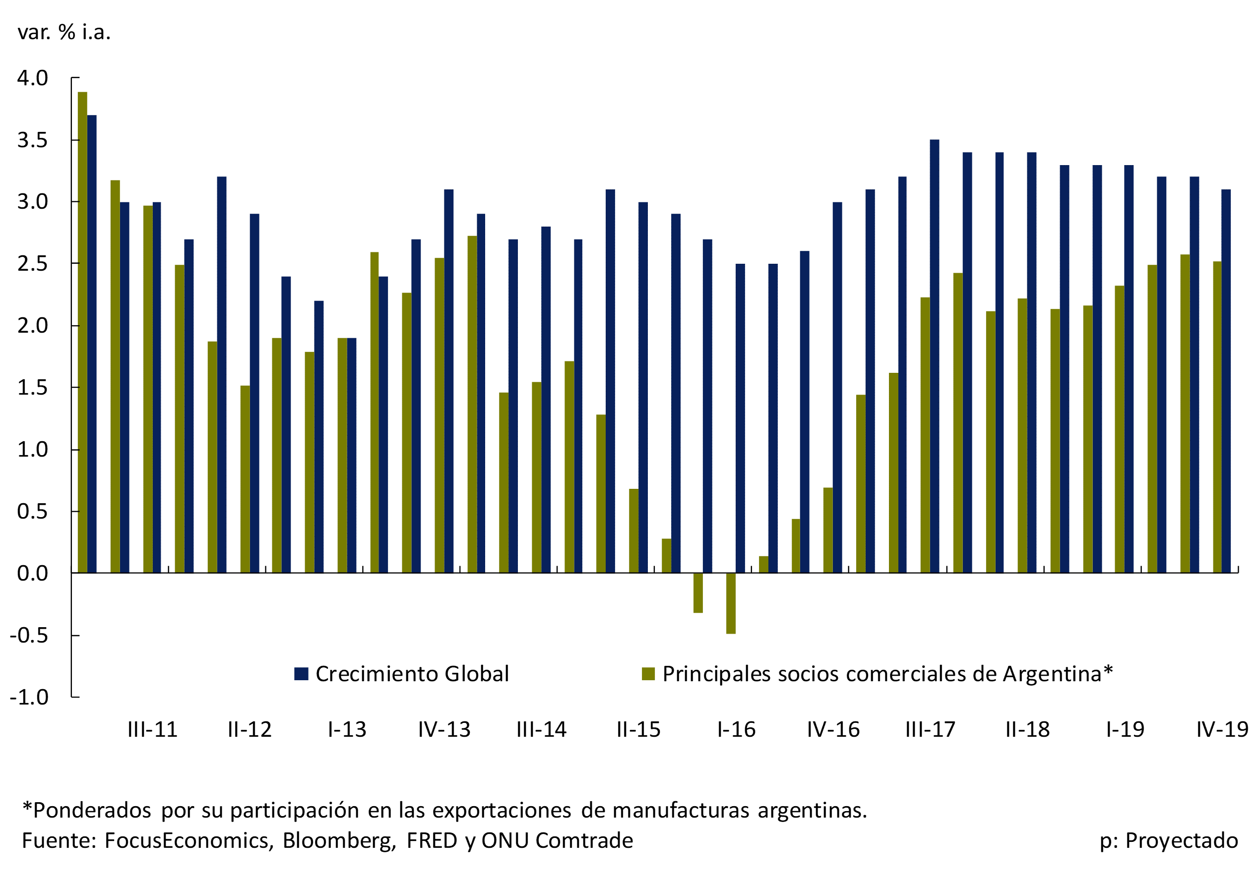
The most recent projections show that the growth rate of the global economy would remain almost unchanged for the remainder of 2018, although growth would be less synchronous than in previous quarters. Thus, the IMF expects world GDP to grow in 2018 0.2 p.p. less than it forecast in July of this year. In the case of Argentina’s main trading partners, their growth rates are expected to continue in the remainder of 2018 at levels similar to those of the most recent quarters, and are expected to reach an eight-year high in 2019 (see Figure 2.1).
Figure 2.1 | Growth of Argentina’s trading partners
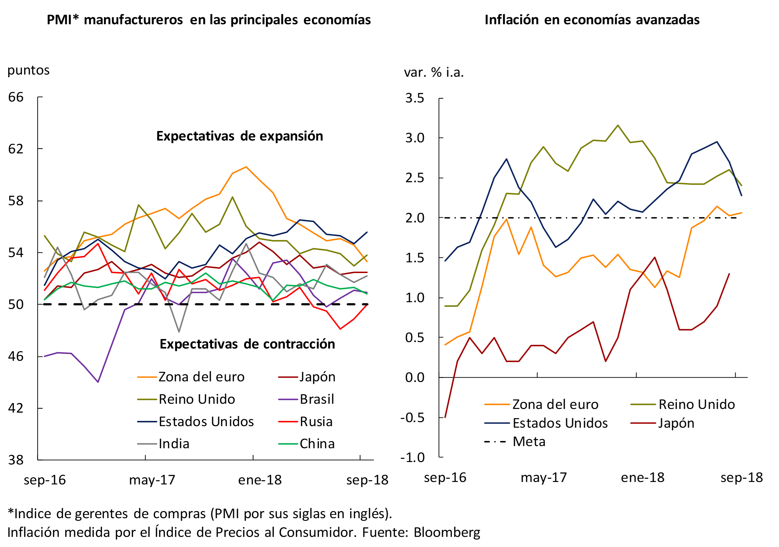
The leading indicators of activity in the main economies are in all cases in the expansion zone. This is in line with inflation data, so the scenario of a more contractionary monetary policy for these economies would be maintained, especially in the case of the United States (see below). Specifically, inflation in the United States and the United Kingdom is 0.3 p.p. and 0.4 p.p. above the target, while in the euro area it is slightly above the target limit (see Figure 2.2).
Figure 2.2 | Leading indicators of manufacturing activity and inflation
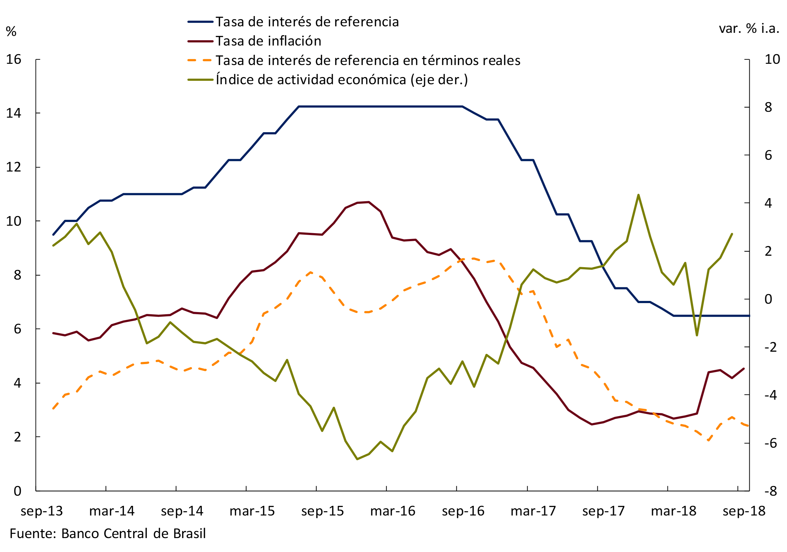
Activity indicators for Brazil, our main trading partner, show that after reaching a low in May (linked in part to union strikes), economic activity has begun to recover. Although the projections for 2018 (Central Bank of Brazil and IMF) continue to be reduced, the increase in the level of activity in recent months would be reflected in 2019, when the highest GDP growth rate in the last five years is projected. Specifically, the projections of the Focus survey – carried out by Brazil’s central bank, BCB, among market analysts – foresee GDP growth of 1.3% for 2018, 0.2 p.p. less than expected at the time of publication of the previous IPOM, while the IMF forecasts a variation of 1.4% (reduction of 0.4 p.p.). For 2019, a GDP growth rate of 2.5% is expected according to Focus and 2.4% according to the IMF.
For its part, in the context of the electoral process in Brazil, the volatility of the exchange rate increased: from the beginning of August to mid-September, the Brazilian real depreciated 13%, and then reversed that depreciation. In the quarter, the BCB made no changes in the monetary policy interest rate, which stands at 6.5% (see Figure 2.3). For its part, despite the fact that inflation in September was the highest since March 2017 (4.5% year-on-year -y.o.y.), it has remained around the center of the target range (4.5% ± 1.5) for four months. Until June of this year, the year-on-year inflation rate was below 3%, having increased in that month by 1.5 p.p. (again linked to the impact of the union force measures). According to the projections of analysts revealed by Focus, inflation would end the year at 4.4%, and at 4.2% in 2019, while the BCB would keep the monetary policy rate unchanged for the rest of 2018, to increase it to 8% in 2019.
Figure 2.3 | Brazil. Macroeconomic indicators
In the euro area, the second destination for Argentine exports, the slowdown in growth that began at the beginning of the year continued, due, according to the European Central Bank (ECB), to a lower level of international trade (lower exports of industrial and capital goods). This was boosted by the appreciation of the euro at the beginning of 2018. However, according to the latest projections, the level of activity in the euro area is expected to stabilise at around 0.4% quarterly growth for the remainder of 2018 and 0.5% for 2019. Labor market data for August show an unemployment rate of 8.1%, the lowest value since November 2008.
Throughout the quarter, the ECB did not modify its monetary policy interest rate, which it applies to Main Refinancing Operations, which remains at an all-time low of 0%, nor did the rate corridor. In addition, no changes in monetary policy interest rates are expected for the remainder of 2018, nor for most of 2019. In addition, the ECB kept its inflation projection for 2018 unchanged at 1.7%, and also at 1.7% for 2019. Finally, the ECB maintains its decision to end its quantitative easing programme at the end of the year, which it has been reducing throughout 2018. 1
Figure 2.4 | USA. Disaggregated change in GDP
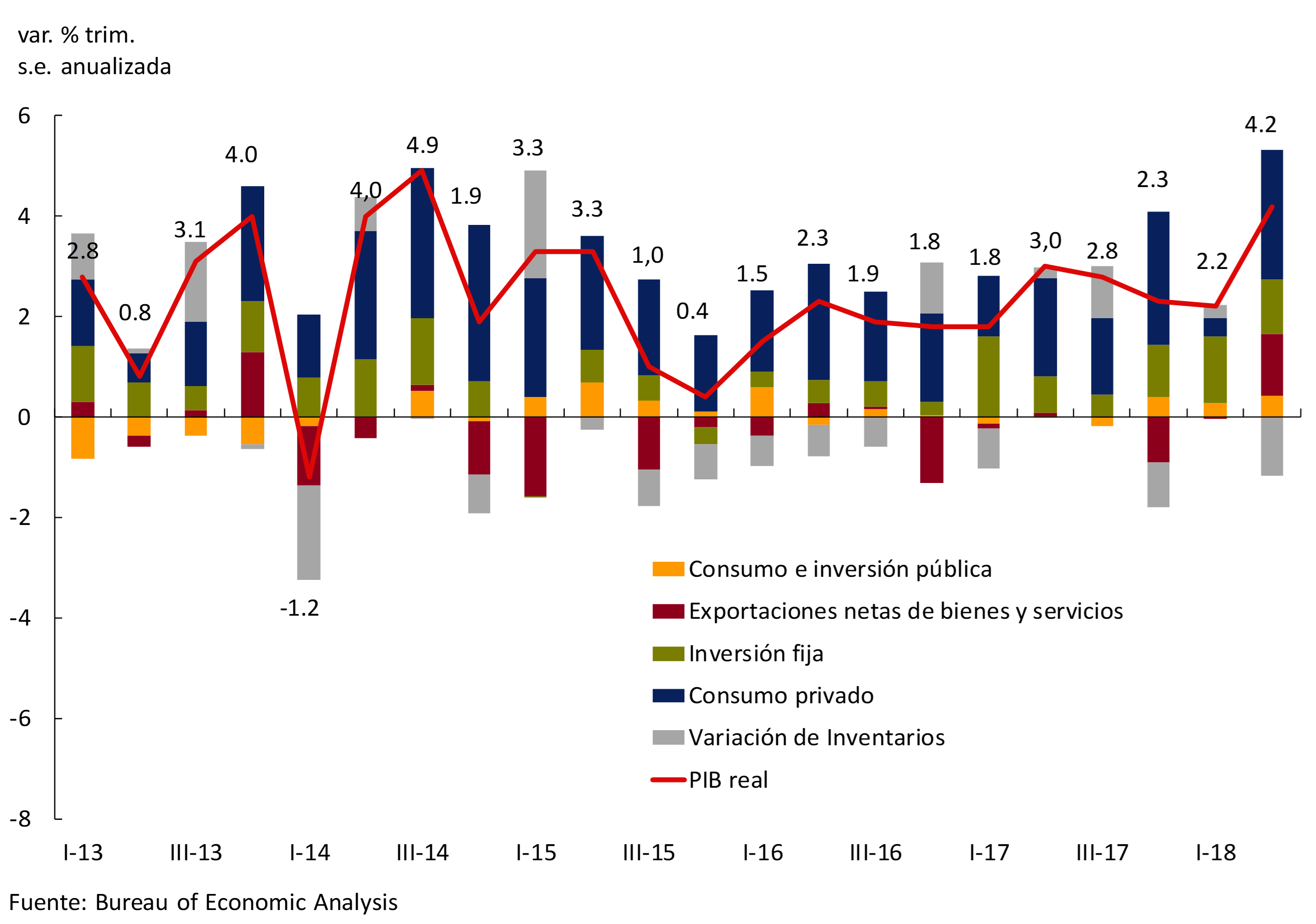
In the United States, Argentina’s third largest export destination , the growth rate in the second quarter was 4.2% (seasonally free and annualized), the highest in the last four years (see Figure 2.4). This was mainly due to the contribution of private consumption – which went from a contribution to growth of 0.3 to 2.6 p.p. – and exports, which contributed 1.2 p.p. Some leading indicators such as the Atlanta Federal Reserve’s GDPNow are showing that the growth rate of the US economy in the third quarter would also be around 4.2%. The higher growth rates that the U.S. economy is registering are linked to the recent fiscal stimulus, which would cease to have an impact on growth in 2020.
Figure 2.5 | USA. Inflation and labour market indicators
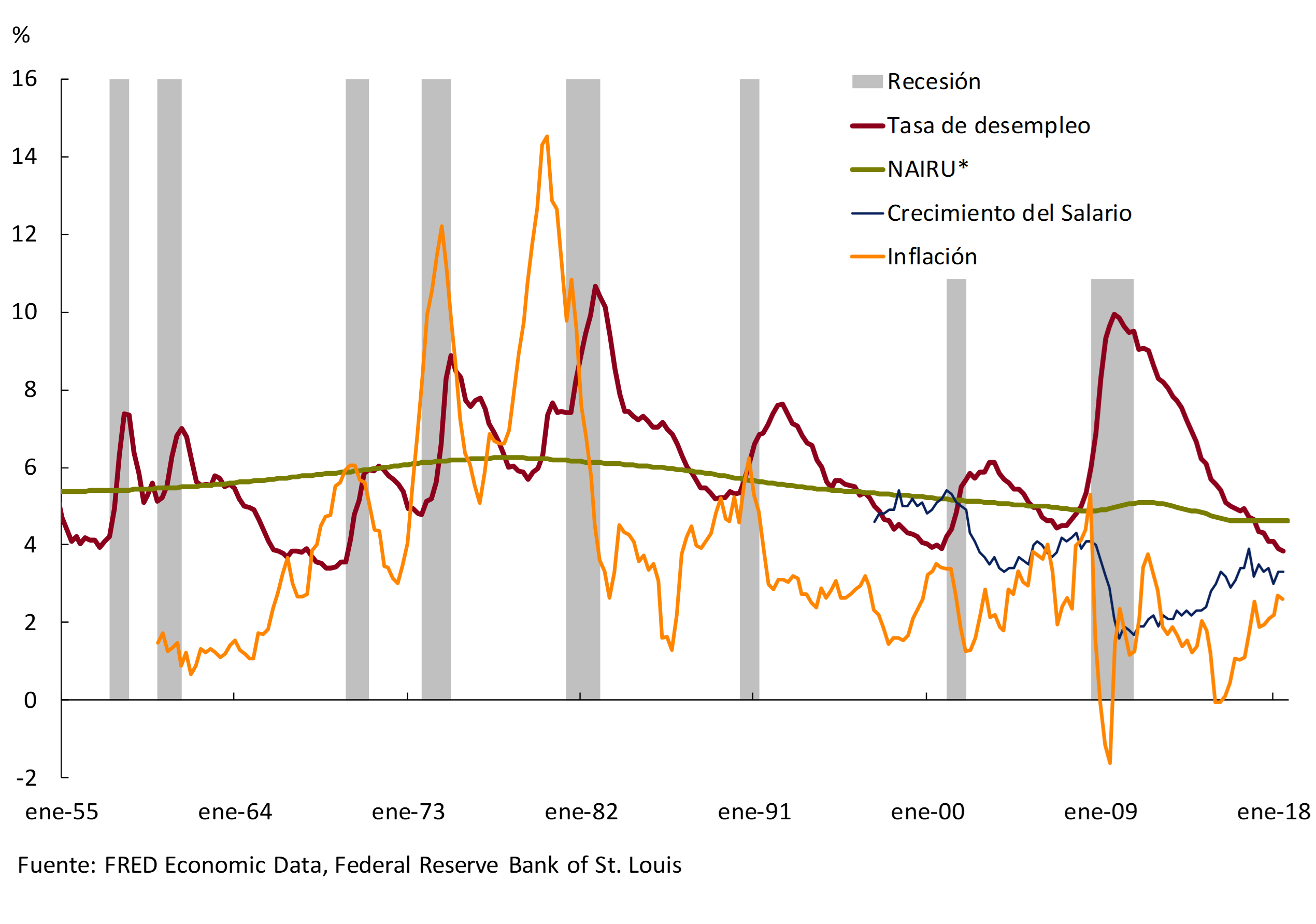
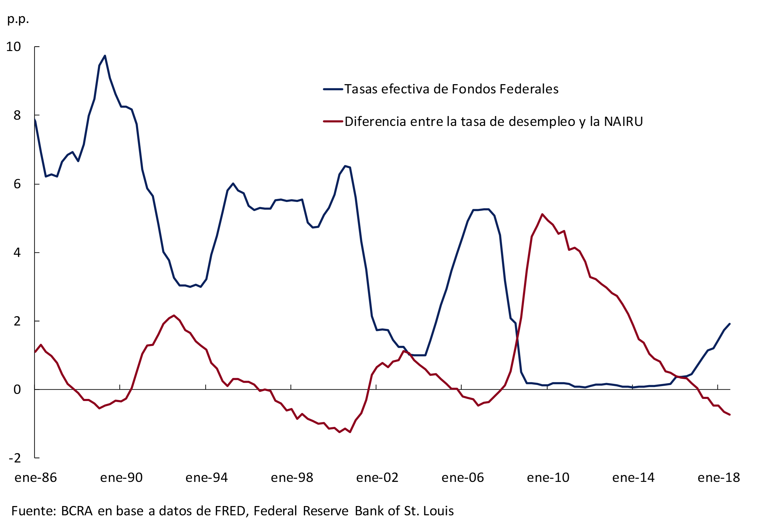
In the case of the labor market, there has been an acceleration in wage increases. In turn, the unemployment rate stood at 3.7% in September (the lowest since August 1969, see Figure 2.5) and -0.9 p.p. below the NAIRU2 estimate, something that had not happened since 2001. At that time, the Fed’s benchmark rate was at values that were more than double the current ones, which could be a sign that the Fed would still have enough room to continue raising its monetary policy rate (the message is even stronger if the benchmark interest rate is taken into account in real terms). In any case, it should be taken into account that the need for the Fed to raise the interest rate may be less if during this time there have been structural changes that have increased the potential GDP of the United States (something that can be inferred from Figure 2.3 of the IPOM of April of this year). Also, the contractionary bias implicit in the benchmark interest rate may be underestimated because it does not take into account the contractionary effect of the end of unconventional monetary policies (asset purchase program).
The Fed’s Monetary Policy Committee (FOMC) increased the benchmark interest rate3 again at its September meeting to the 2-2.25% range. In addition, from the latest projections released by the FOMC, it is expected to increase its benchmark interest rate once again in the remainder of 2018 to the range of 2.25-2.5%. Thus, by the end of 2018 the benchmark interest rate in real terms would be positive again for the first time in more than a decade (since September 2008). In this regard, in its press release , the FOMC stopped describing its monetary policy as expansionary. In addition, the FOMC’s projections also show that three increases in the benchmark interest rate are expected during 2019 (0.25 p.p. each time). There were no significant changes in the case of the activity (growth and unemployment) and inflation projections. Thus, GDP is expected to grow 3.1% and 2.5% in 2018 and 2019, unemployment to be 3.5% (in both years), and inflation to be 2.1% and 2% respectively.
Figure 2.6 | USA. Fed benchmark interest rate against the NAIRU
Growth in China, the main destination for Argentina’s exports of primary products, slowed during the third quarter. This data does not yet register the full impact of the trade tariffs imposed on its exports to the United States. Specifically, during the third quarter GDP increased 6.5% year-on-year (0.2 p.p. less than the second quarter). In this context, a few days earlier the Central Bank of China had ordered a reduction in reserve requirements on the financial system. In this way, it would seek to prioritize growth over the deleveraging policy that China has been carrying out. The most recent projections for 2018 show expected GDP growth of 6.6% for this year and 6.2% for 2019 (unchanged for 2018, and 0.2 p.p. less for 2019 than previous projections). Finally, the Chinese yuan, which had depreciated sharply against the dollar since mid-June, was relatively more stable, having depreciated from the values in force at the time of publication of the previous IPOM (3.3%).
2.2 The tightening of the external financial scenario continued, although at a slower pace than in the previous quarter
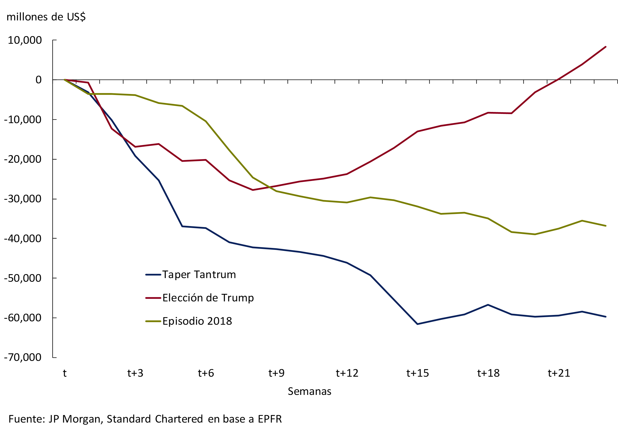
In the third quarter, the external financial scenario continued to tighten, worsening global liquidity conditions for emerging countries, and for Argentina in particular, although at a slower pace compared to the second quarter. Thus, both the depreciation of emerging market currencies and the increase in sovereign risk premiums continued, as a result of capital outflows from these markets (see Figure 2.7). As noted in the previous IPOM, those economies with external imbalances and/or high levels of indebtedness were particularly affected. However, it should be noted that global liquidity conditions, despite the recent deterioration, remain comfortable in historical terms.
Figure 2.7 | Emerging Markets. Capital flows
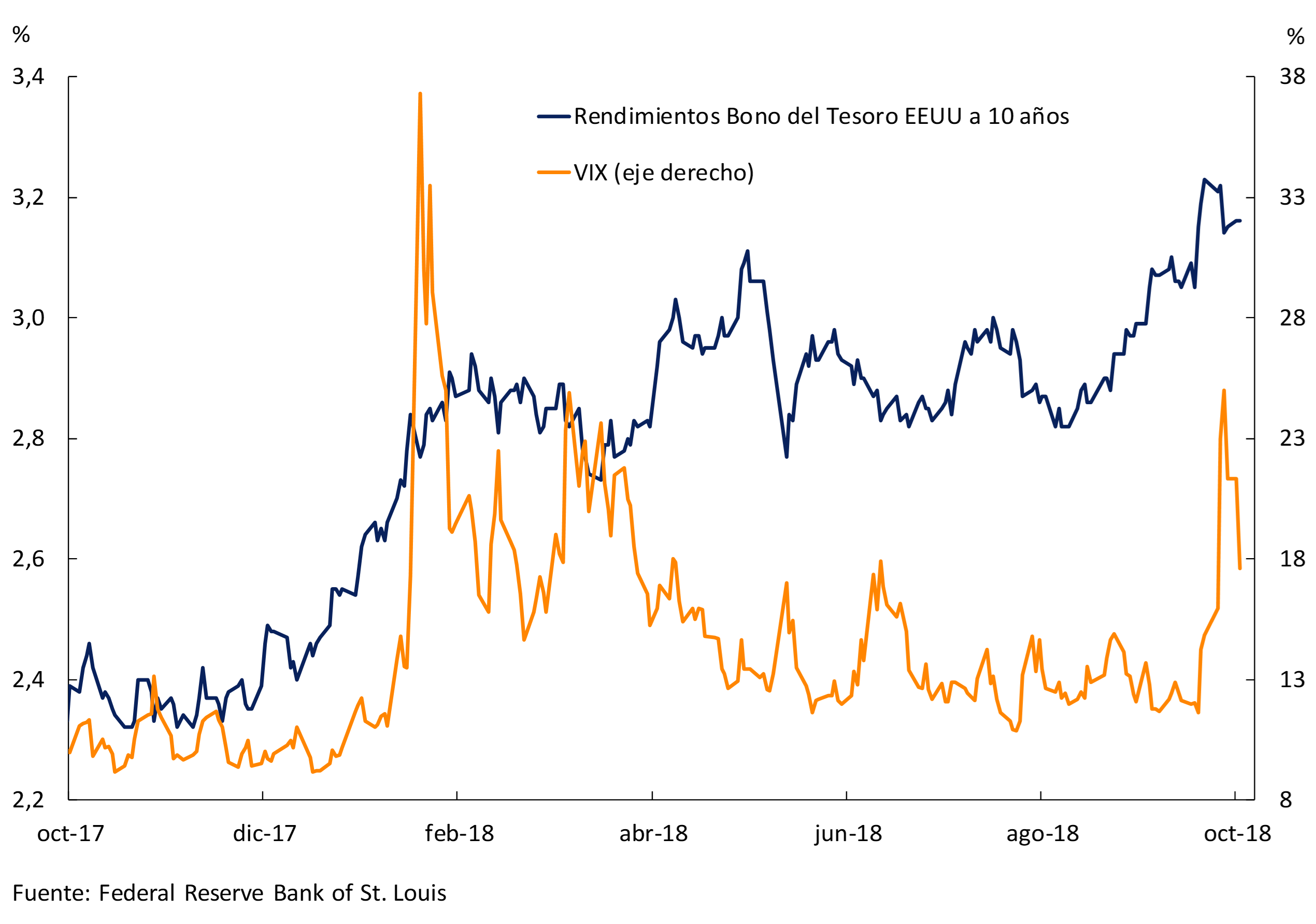
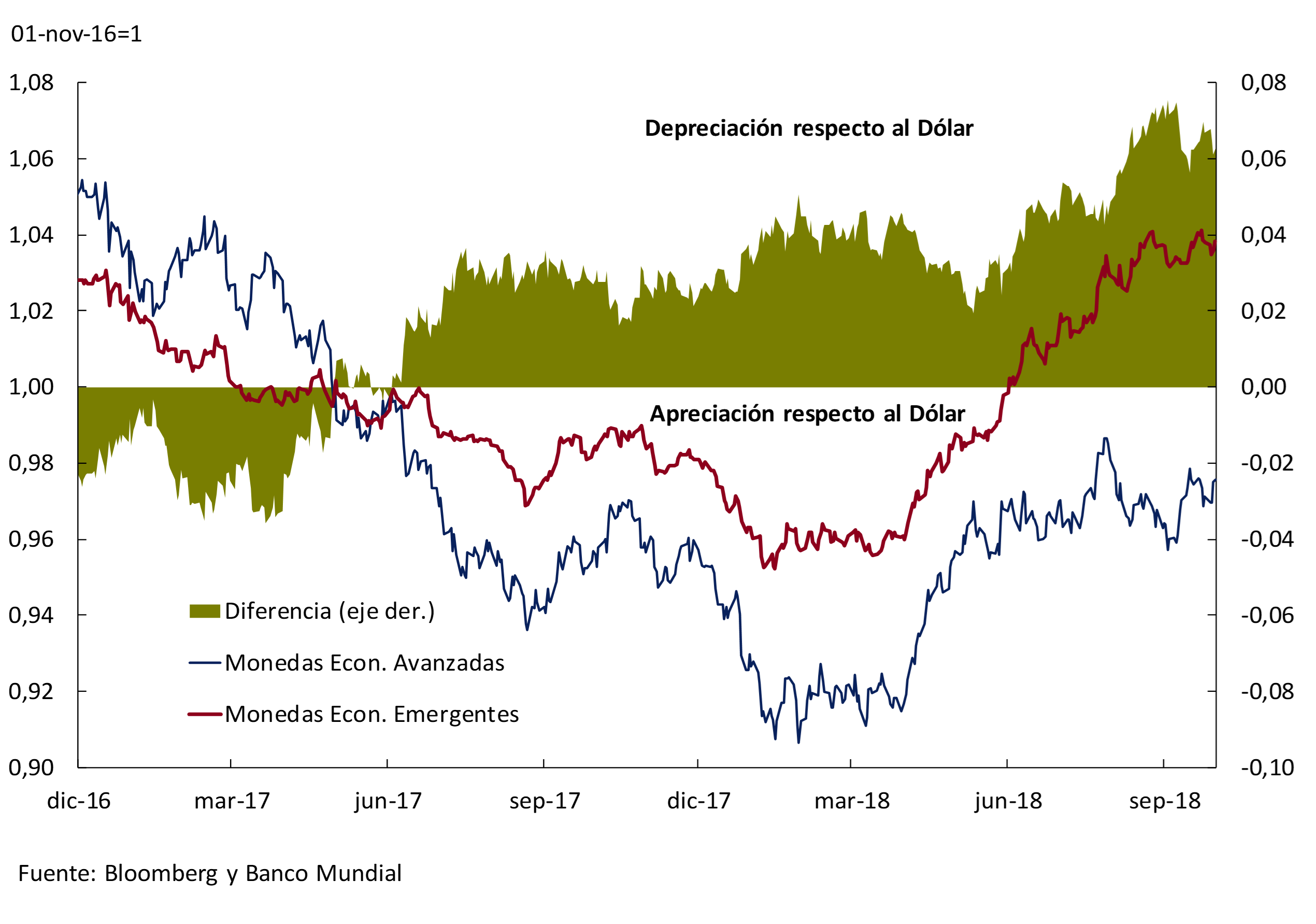
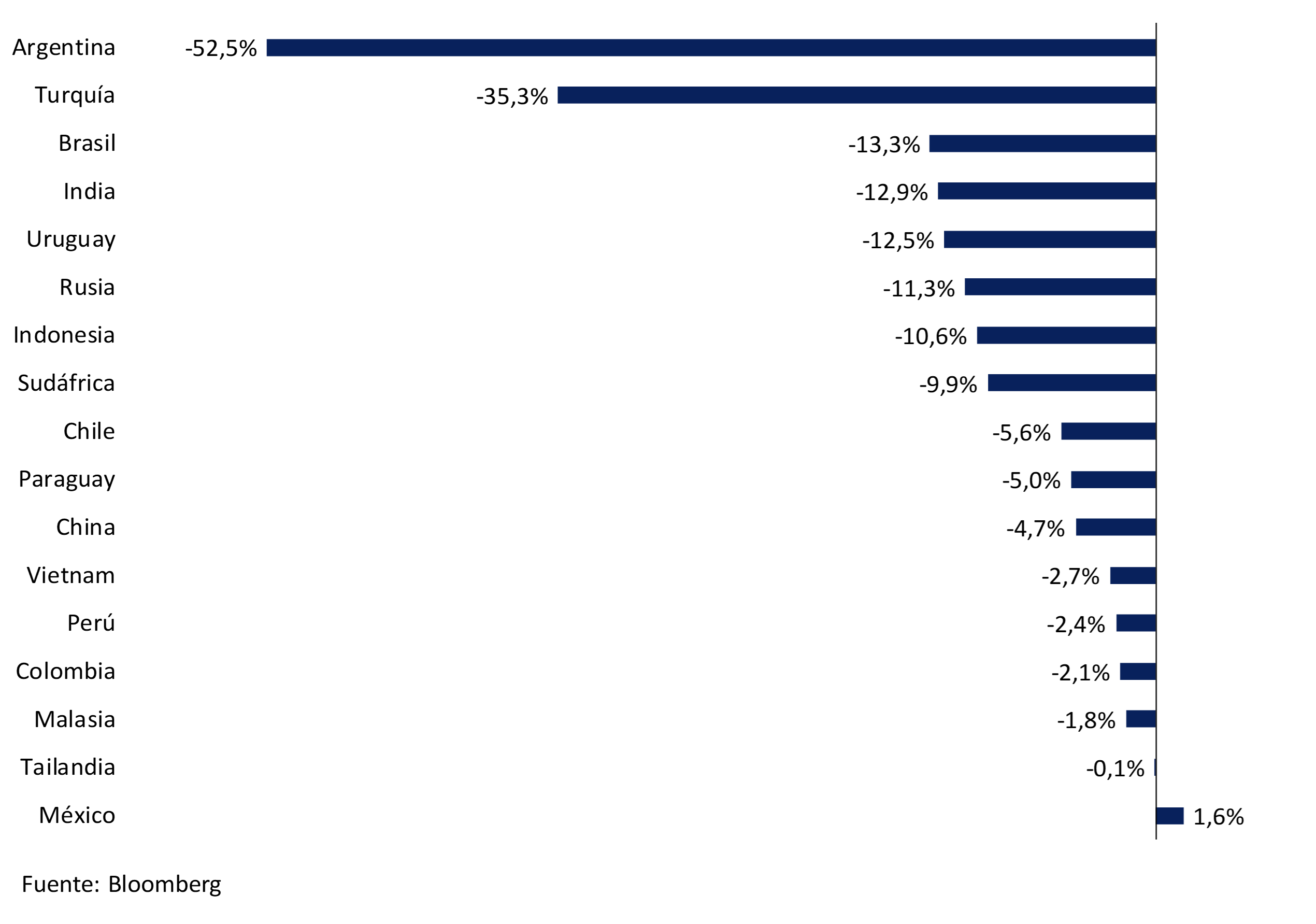
The tightening of monetary conditions in the United States can be seen in the increase in the interest rate on the ten-year U.S. treasury bond (see Figure 2.8), which began in December 2017. Since April, the rise in the performance of this benchmark began to coincide with an appreciation of the dollar (see Figure 2.9), which increases the adverse effect on emerging markets. Then, since mid-August, the increase in the rate of the ten-year bond accelerated. In this context, Argentina and Turkey were the countries that suffered the sharpest depreciations in their currencies (see Figure 2.10). There were other economies that were affected by the international context, but also by idiosyncratic factors, such as Brazil and South Africa.
Figure 2.8 | Financial market indicators
Until August 9, the Turkish lira accumulated a depreciation of 31.6% in the year. On that day, the United States doubled tariffs on steel and aluminum imports from Turkey, arguing that it should protect itself from the use of the exchange rate as a competitive tool. This led to further depreciation of the lira. With a persistent current account deficit since 2002 (5.4% of GDP estimated for this year), Turkey accumulated external debt and relies on new financing to cover the external gap. To face the unfavorable external context, it indirectly tightened monetary conditions and sought financial assistance outside international organizations, obtaining support from Qatar. Then, in mid-October, the Turkish government placed debt again on international markets.
Figure 2.9 | Depreciation of emerging currencies vs. advanced economies
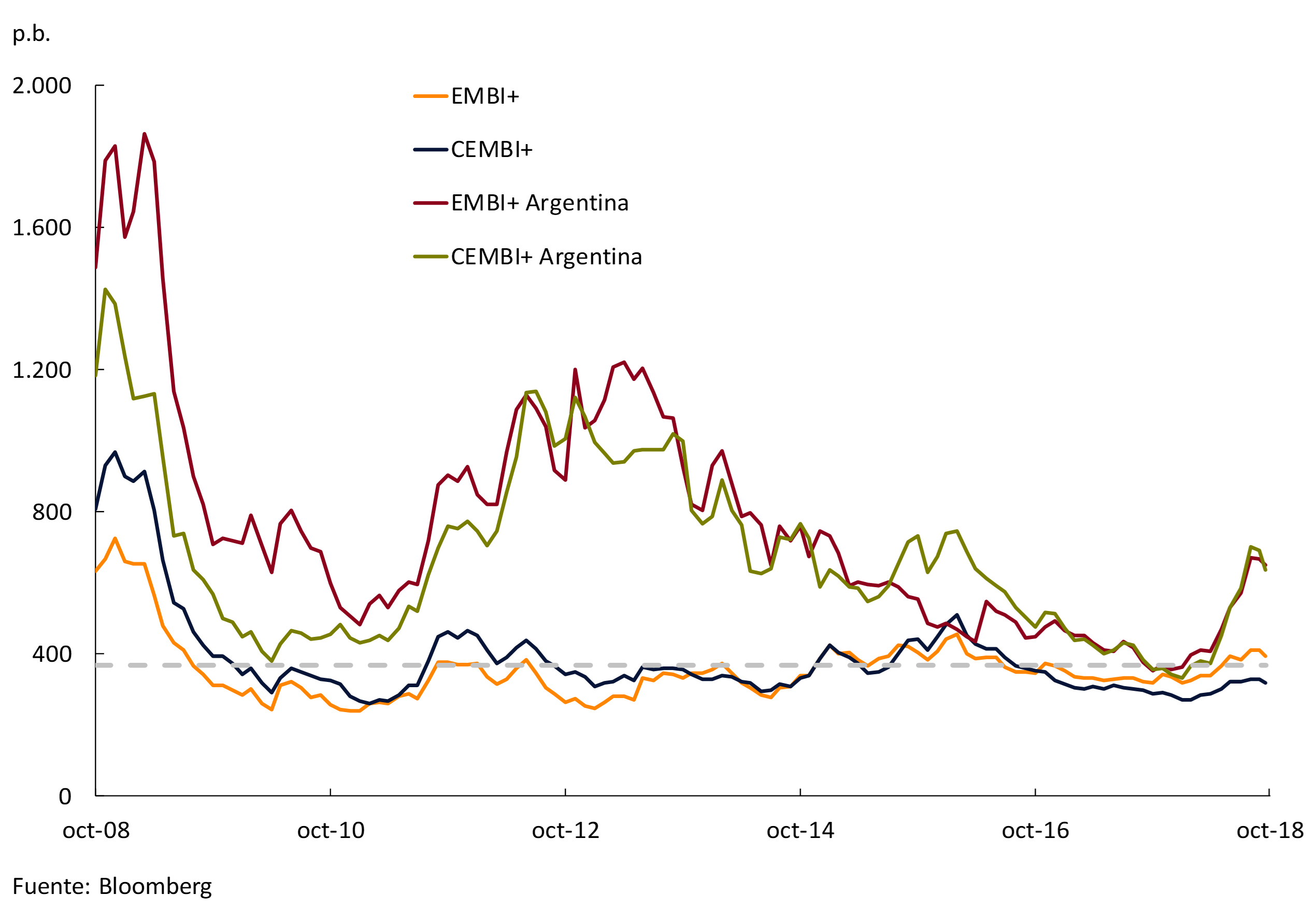
During the third quarter of 2018, emerging countries faced higher sovereign risk premiums than in recent years, although they registered a decrease in the margin. Corporate risk premiums for emerging economies remained relatively stable compared to the previous quarter – still around the lows of recent years – but were above 2017 levels. In a context in which the cost of external financing continued to increase, the amount of gross sovereign and corporate debt issuances of emerging countries in international markets registered a decrease of 42% year-on-year in the third quarter. The contraction was stronger in sovereign issuances, accounting for a 77% year-on-year drop, while corporate issuances showed a 31% year-on-year drop.
Figure 2.10 | Depreciations of emerging currencies. October 2018 vs. December 2017
For Argentina, external credit conditions showed a significant deterioration in relation to the second quarter. Argentina’s sovereign and corporate risk premiums rose to levels recorded in 2015, with widening of the relative gaps with respect to the rest of the emerging economies, although there was a slight improvement in the margin (see Figure 2.11). Regarding Argentina’s sovereign placements abroad, no operations were registered during the third quarter of the year. With the CEMBI+ARG (Argentine Corporate Emerging Markets Bond Index) averaging 670 points, there were no issuances in foreign markets by Argentine companies. In fact, the last placement dates from the end of April, before the beginning of the financial turbulence.
Figure 2.11 | Sovereign and corporate debt risk indicators
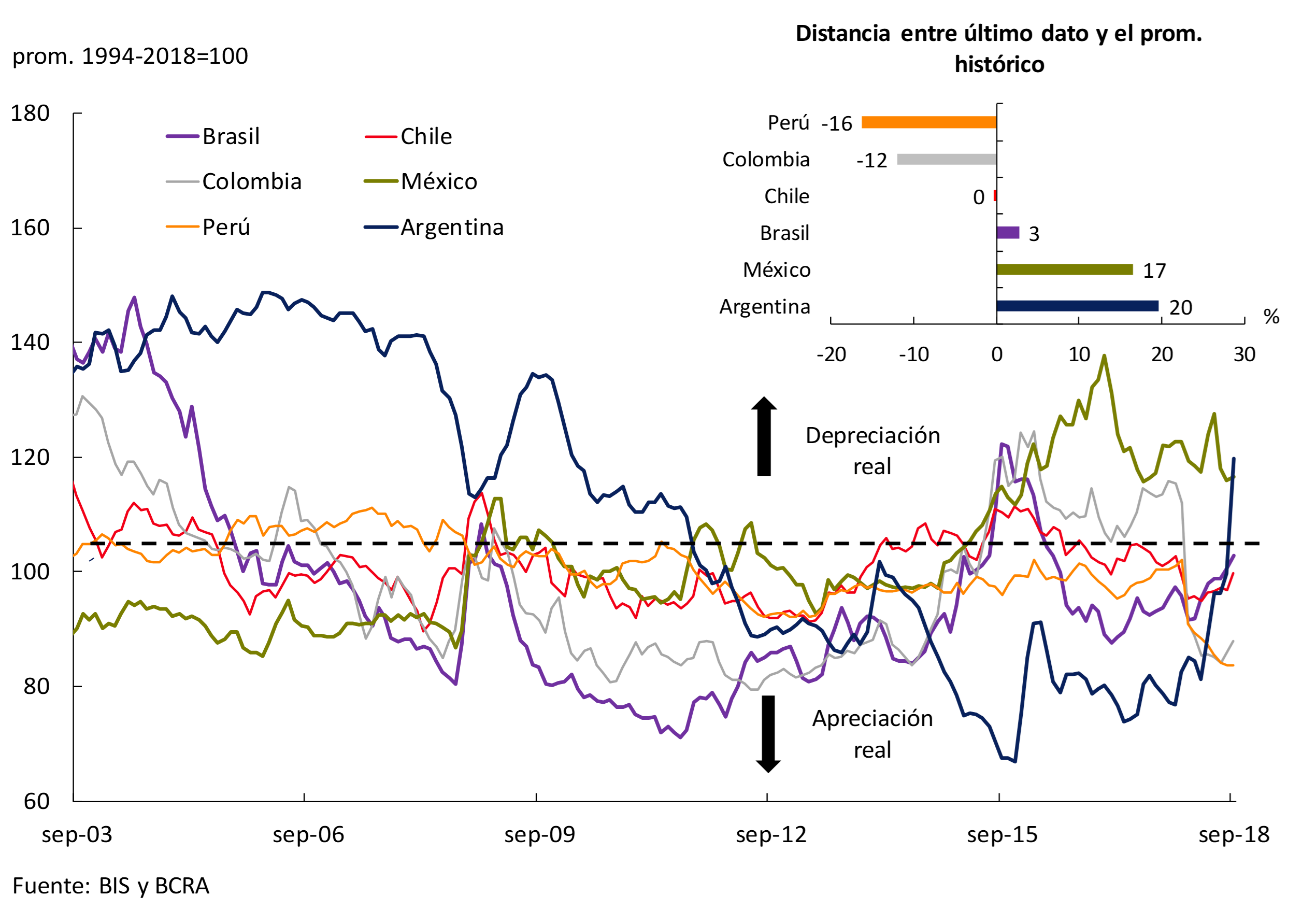
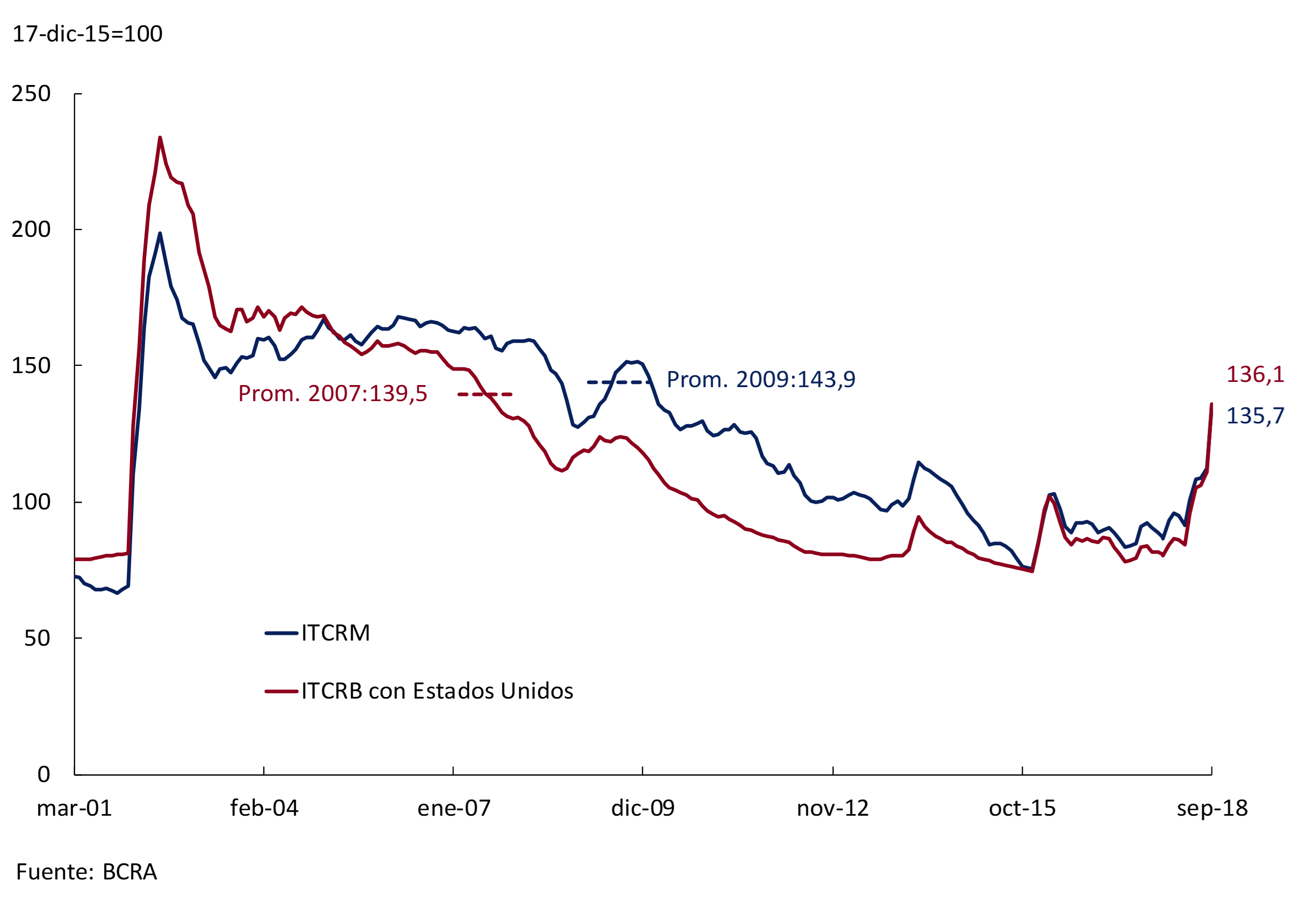
In the third quarter, the Multilateral Real Exchange Rate Index (ITCRM) rose 18% on average compared to the second quarter, mainly due to a nominal depreciation of the peso against the dollar. The end-to-end increase was even greater, 24%. Thus, in September, the ITCRM was 21% above the average of the last twenty-four years (see Figure 2.12). In comparison with other countries in the region, the peso is the currency that has depreciated the most compared to its historical average, which gives domestic goods a marked improvement in price competitiveness. This situation has not occurred since the beginning of 2012, when Argentina registered a trade surplus of goods of around 2% of GDP.
Figure 2.12 | Multilateral Real Exchange Rate
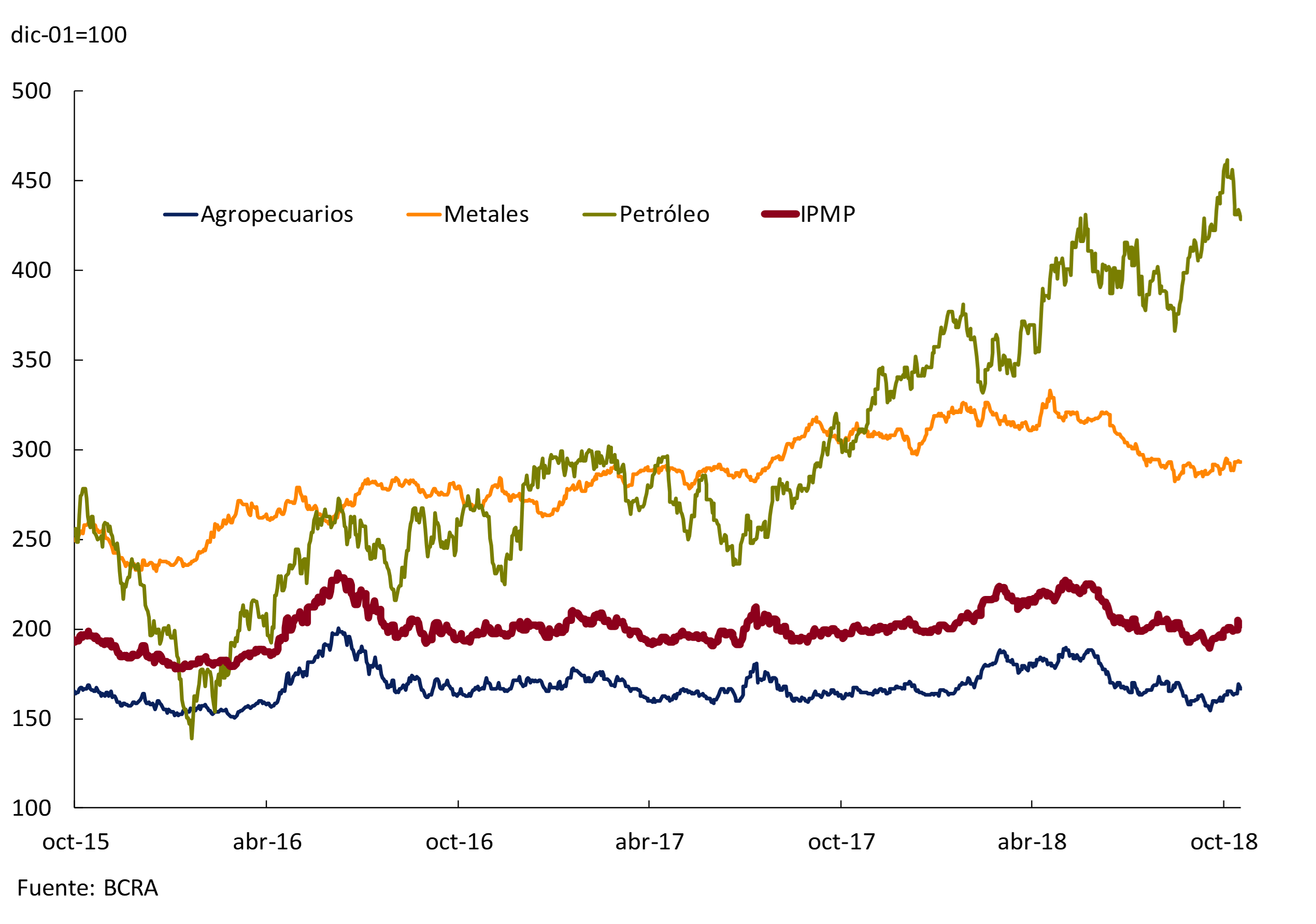
On the other hand, international commodity prices measured in dollar4 continued to decline in the third quarter, implying values that at the margin are approximately 1% below the levels of the same period of the previous year. Prices of agricultural products and metals rose in October, unlike the international price of oil, which fell slightly, although it remained around the highest levels in recent years (see Figure 2.13).
Figure 2.13 | International commodity prices
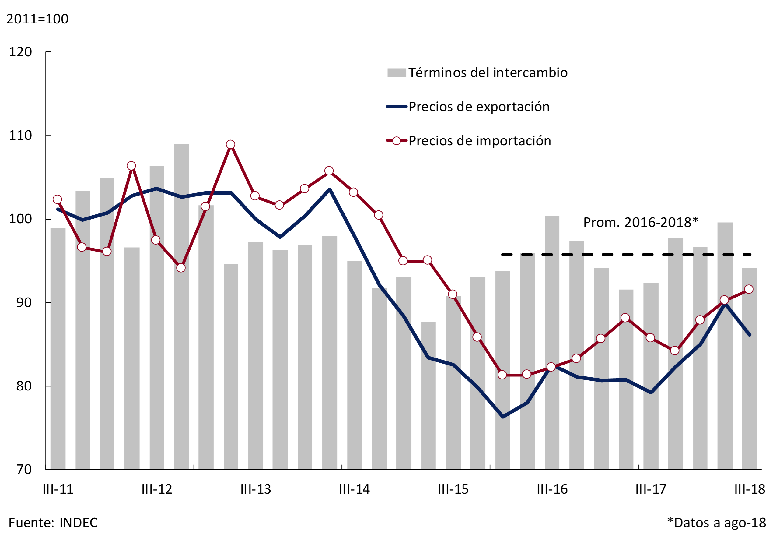
Finally, as anticipated in the July IPOM, the terms of trade (quotient between the prices of Argentine exports and imports)5 fell 4.1% in the July-August two-month period, as a result of a fall in the price of exports and an increase in the price of imports – influenced by the upward trend in the international price of crude oil. This evolution was influenced by both the decline in the price of soybeans as a result of the trade disputes between China and the United States and the rise in the price of oil (see Figure 2.14).
Figure 2.14 | Terms of Exchange
In summary, the deterioration of international financial conditions continued in this quarter, although at a slower pace compared to the second quarter. The good performance (current and projected) of the level of activity of our main trading partners could offset the adverse financial scenario, configuring a mixed external scenario for Argentina. The main risks of this scenario are the continued tightening of international financial conditions6 and a deepening of protectionist measures7. This would deteriorate the external situation of emerging countries, with an impact on the level of activity of our trading partners.
3. Economic activity
In the second quarter, the economy contracted in line with the adverse scenario foreseen in the previous IPOM. During the third quarter, the fall in non-agricultural output deepened in the face of a greater than expected deterioration in domestic financial conditions.
Consumption and investment, both public and private, fell again while net exports contributed positively to the quarterly variation in output. At the sectoral level, the fall was widespread, partially offset by the normalization of agricultural activity and the growing trend of some activities such as livestock, oil and gas.
The decision of the Executive Branch to accelerate convergence to the primary fiscal balance and the advancement of the disbursements foreseen within the framework of the agreement with the IMF allow clearing up the uncertainty installed in the financial markets regarding the government’s financing needs. It is expected that after the initial contractionary impact of the depreciation, the higher real exchange rate will begin to give impetus to tradable sectors during 2019 and contribute to the reversal of the current account imbalance.
Although the economic outlook deteriorated compared to the previous IPOM, the BCRA continues to expect that the correction of the external and fiscal deficits will allow a recovery to begin during 2019 on a more sustainable basis.
3.1 The economy will contract in 2018
During the second quarter, GDP fell 4% s.e. and 4.2% y.o.y. in line with the adverse scenario foreseen in the previous IPOM. The fall in “non-agricultural” GDP (-1.1% quarter-on-quarter s.e.) is explained by the contraction of domestic demand as a result of financial tensions that led to an abrupt jump in the exchange rate, with the consequent increase in inflation, the fall in real wages and the increase in uncertainty. Transport and trade also suffered the indirect impact of the drought that strongly affected agricultural products.
During August, the dollar strengthened globally and the prices of financial assets in emerging economies deteriorated. The new international shock depreciated the currency of Brazil, our main trading partner, decreasing its expected growth rate for 2019. The perception of risk on the vulnerabilities of the Argentine economy increased, leading to an additional portfolio rebalancing and a new depreciation of the peso, not contemplated in the macroeconomic assumptions of the previous IPOM base scenario. The increase in inflation during August and September deteriorated real wages, explaining the deepening of the fall in domestic demand during the third quarter. In this context, the BCRA adopted a new monetary policy framework in order to limit exchange rate instability and contain price rises (see Monetary Policy Chapter).
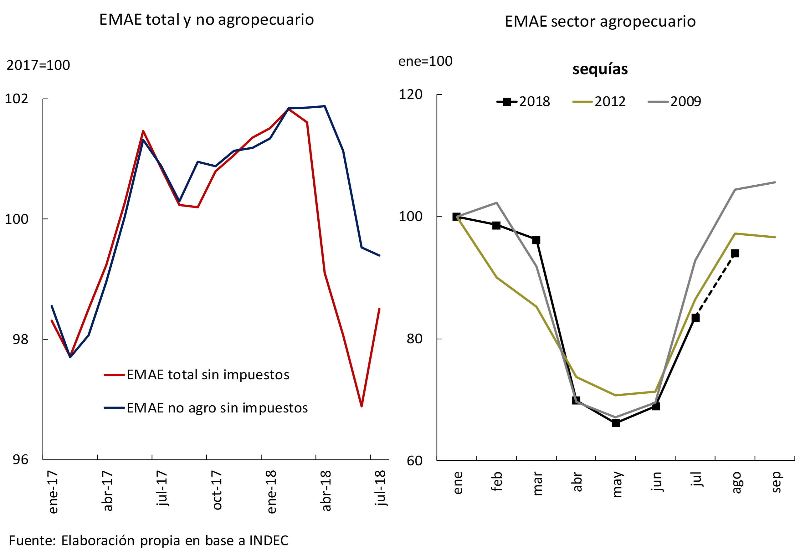
In a more adverse context than expected, non-agricultural output declined in the third quarter, while the normalization of agricultural activity contributed approximately 2 percentage points (p.p.) to the quarterly variation in GDP, partially offsetting the contraction of the rest of the sectors. The available data are in line with that forecast. INDEC’s Monthly Estimator of Economic Activity (EMAE) increased 1.4% s.e. in July, explained by a 26% s.e. recovery of the agricultural sector compared to June (see Figure 3.1). The General Activity Index of O.J. Ferreres also increased in July due to the effect of agriculture (4.5% monthly s.e.) and remained stable in August. The latest Contemporary BCRA GDP Prediction (PCP-BCRA) for the third quarter indicates a fall of 0.5% quarter-on-quarter s.e.
Figure 3.1 | Monthly evolution of economic activity
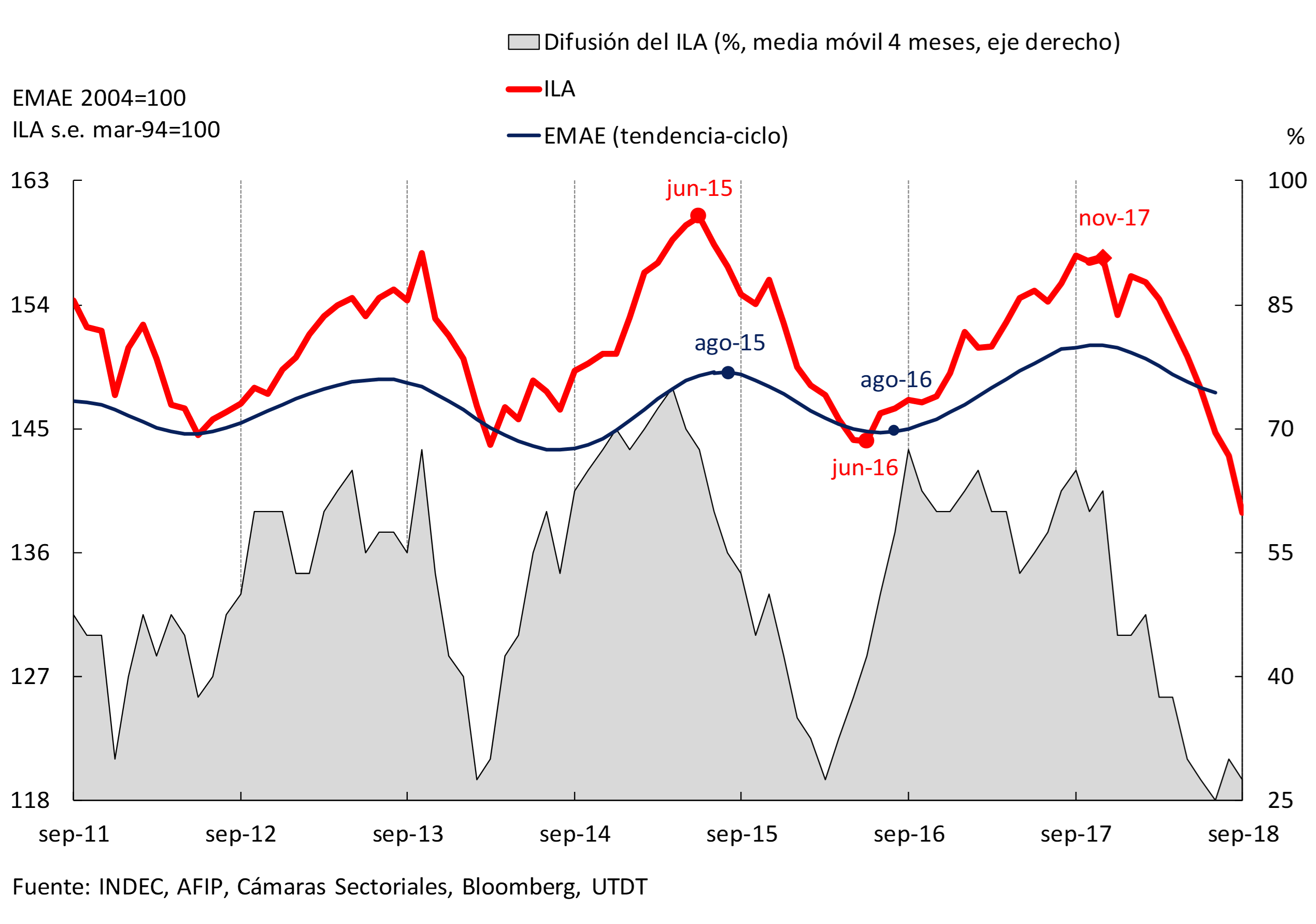
For the rest of the year, the Leading Indicator of Activity (ILA-BCRA) does not allow us to anticipate a change in the recessionary phase that began in the second quarter of 2018. In September, the ILA recorded the seventh consecutive monthly decline and the growth spread stood at 27.5%, close to historical lows8 (see Figure 3.2).
Figure 3.2 | Leading Activity Indicator (ILA)
The BCRA’s new monetary policy framework seeks to moderate exchange rate volatility and gradually reduce inflation. For its part, the Executive Branch decided to accelerate the process of fiscal consolidation, a necessary condition to reduce the cost of financing and reduce financial and exchange rate instability. Towards the end of September, a new agreement was reached with the IMF technical team with the aim of clearing up uncertainty about the 2019 financial program. In the coming months, the economy will go through the correction of the external and fiscal deficits, allowing a recovery to begin during 2019 on more sustainable bases.
3.1.1 Domestic demand reflected the deterioration of financial conditions from the second quarter onwards, adding to the fall in agricultural exports
In the second quarter of 2018, the sharp drop in domestic demand (-2.1% s.e.) was added to the contraction in exports explained by the drought that affected soybean and corn production. 9 The lower foreign exchange inflow due to the supply shock in the agricultural sector, together with the deterioration of financial conditions and the sharp increase in the exchange rate, affected real wages, causing a contraction in private consumption (-1.1% s.e.) and investment (-6.9% s.e.). Leading indicators allow us to anticipate that the contraction in domestic demand continued in the third quarter.
Table 3.1 | Quarterly change in GDP and contributions of its components
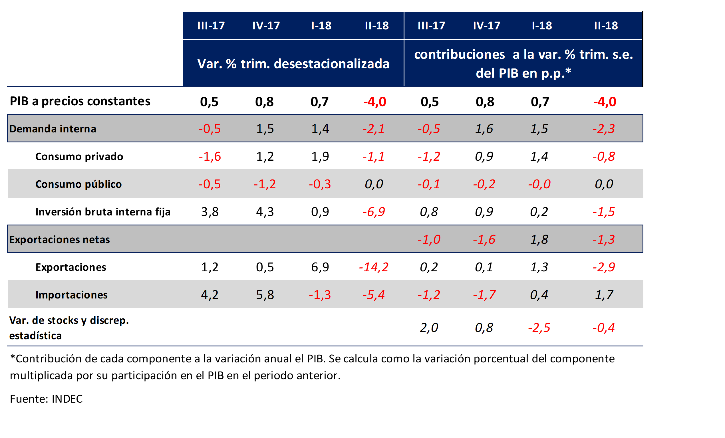
Private consumption was affected by lower households’ real disposable income in a context of tighter credit conditions and deteriorating consumer expectations. The real salary of registered workers fell by an average of 1.7% during the second quarter. Between April and June, national public sector spending on social protection (retirements, pensions, family allowances and other social programs) increased by 28.1% nominal YoY. However, in order to protect the most vulnerable sectors, the government has decided to increase the AUH, making two extraordinary payments to the 4 million beneficiaries. In this way, this item of expenditure would exhibit a growth in real terms of more than 10% during 2018.
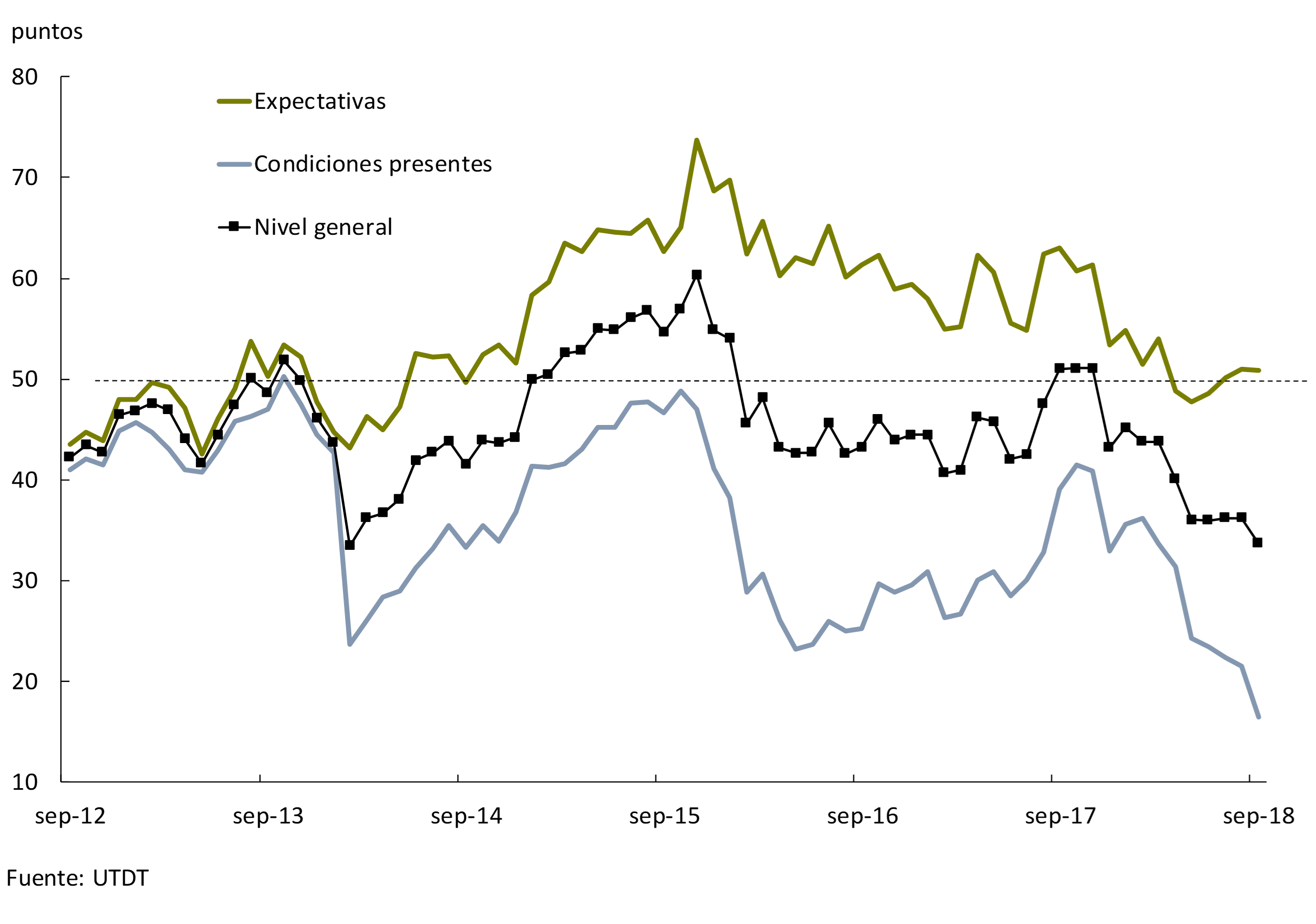
In the third quarter, consumer expectations deteriorated sharply, anticipating a poor performance of consumption. The Consumer Confidence Index (CCI) of the Torcuato Di Tella University was at the lowest level since February 2014 in September, with a 34% drop compared to a year ago (see Figure 3.3). Among the components of the ICC, the main decrease was observed in the predisposition to purchase durable goods and real estate (household appliances, houses and cars), which was more accentuated in the interior of the country.
Figure 3.3 | Consumer Confidence
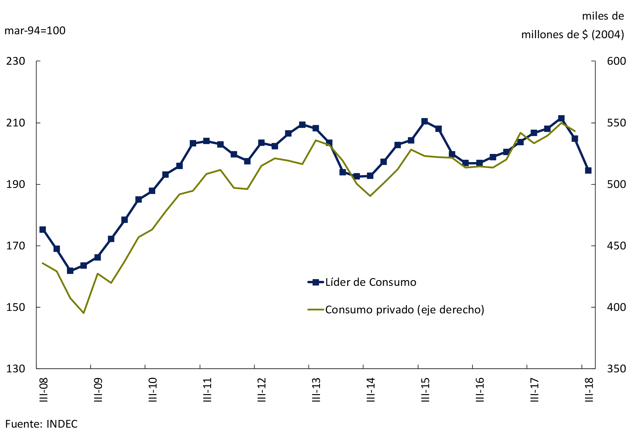
The Coincident Index of Private Consumption prepared by the Undersecretariat of Macroeconomic Programming decreased by 1.7% s.e. in the third quarter, while the BCRA’s Leading Indicator of Private Consumption10 also suggests that the decline in consumption was accentuated between July and August (see Figure 3.4).
Figure 3.4 | Private consumption
It is expected that, in a scenario of greater certainty, private consumption will reach a floor during the first quarter of 2019 in line with the reopening of the parity agreements that will improve real wages with respect to the minimums projected for the fourth quarter of 2018.
Investment decisions were affected from the second quarter onwards by the increase in the relative price of capital goods, the deterioration of domestic financial conditions and the unfavorable outlook for domestic demand. The contraction in gross domestic investment in the second quarter (-6.9% s.e.) had the largest contribution to the quarterly fall in GDP. Among its components, the reduction in durable equipment (-5.7% s.e.) stood out, mainly explained by lower imports of imported transport material (-16.3% s.e.).
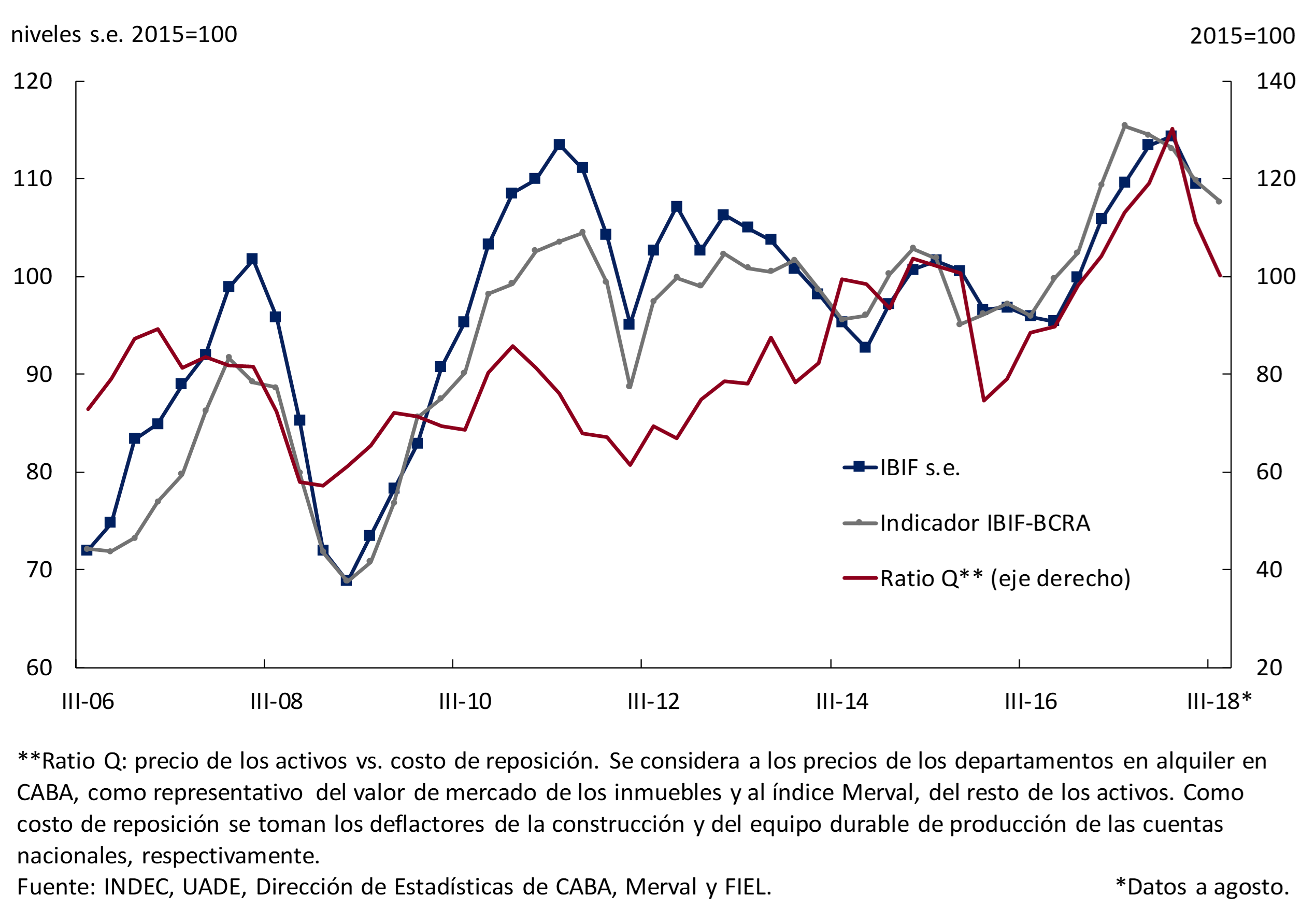
Partial indicators indicate that in the third quarter investment continued to decline. The IBIF-BCRA11 indicator fell 2.3% s.e. compared to the previous quarter, while the Coincident Investment Index prepared by the Undersecretariat of Macroeconomic Programming of the Ministry of Finance shows a fall of 5% s.e. This performance can be anticipated by the Q ratio, which relates the market value of assets to the replacement cost of assets and continued to fall through August (see Figure 3.5).
Figure 3.5 | Investment evolution
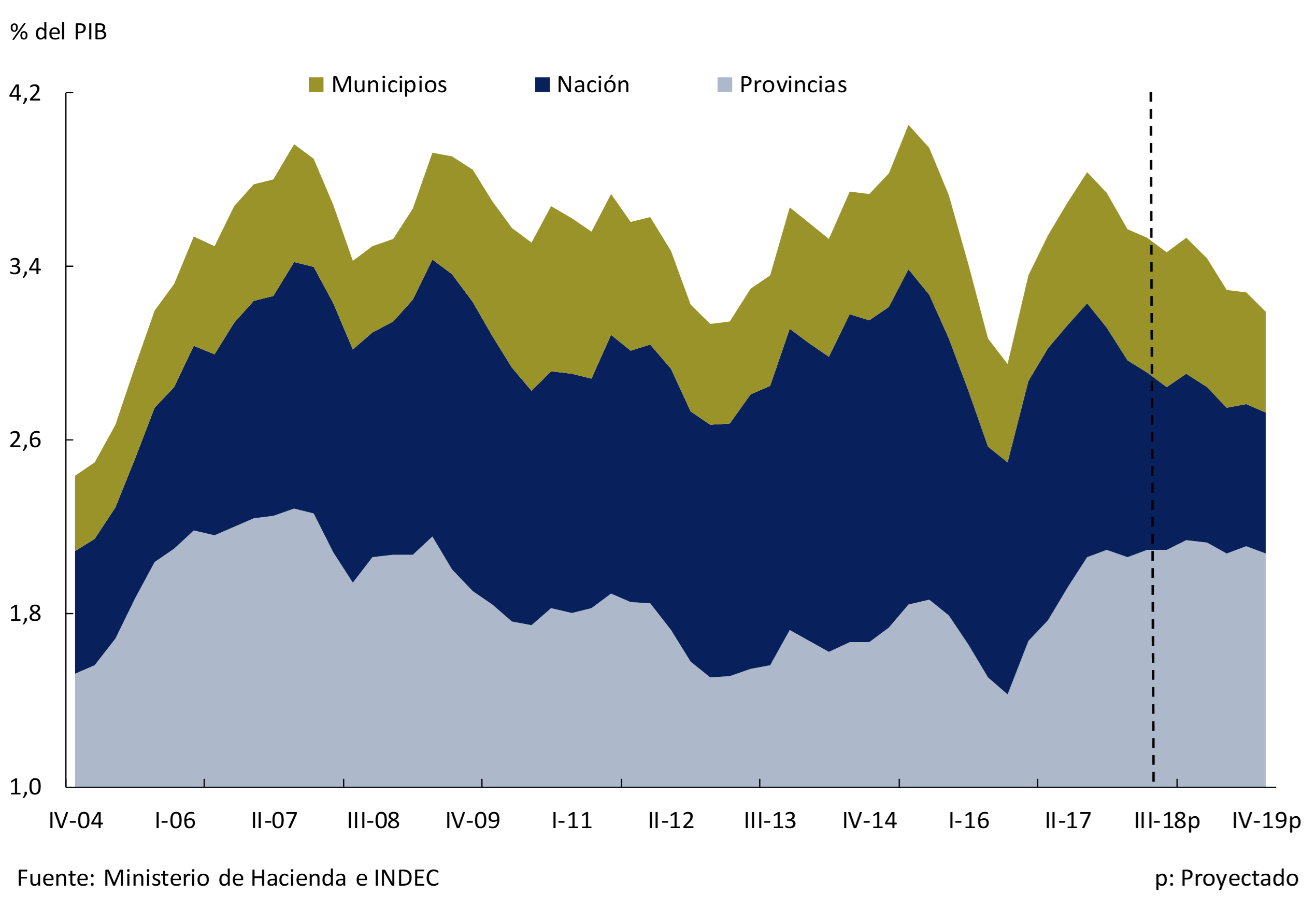
The negative trend in private investment is expected to continue and recover as financial uncertainty clears and the outlook for domestic demand improves. For its part, public investment will have a lower contribution than in 2017 within the framework of the policy of consolidation of fiscal accounts carried out by the Executive Branch. Consolidated public sector capital expenditure is expected to be lower in the second half of the year than in the first half of the year, a trend that is expected to continue in 2019 (see Figure 3.6).
Figure 3.6 | Public sector capital expenditure
One of the main exceptions to the unfavorable dynamics of investment is in the energy sector, especially in the exploitation of wells for oil and gas extraction in the Vaca Muerta formation. Projects in this sector were not affected by the recent financial and exchange rate turbulence, and the outlook for the coming years is encouraging.
The BCRA expects that, as financial conditions stabilize, private investment will begin to recover, led by tradable sectors that are in a position to take advantage of a more competitive real exchange rate.
3.1.2 Net exports would contribute positively to aggregate demand with the normalization of agricultural activity, cushioning the fall in the third quarter
As anticipated in the previous IPOM, there was a sharp drop in the quantities exported of goods and services in the second quarter (-14.2% quarterly s.e.) mainly explained by the lower availability of grains after the drought (soybean and corn complex). In the third quarter, the recovery of agricultural exports added to the positive trend evidenced by the rest of exports since the end of 2015. Imports of goods and services fell 5.4% quarter-on-quarter in the second quarter, due to the impact of the recession and the increase in the real exchange rate. This drop was accentuated between July and September.
The quantities exported of cereals, oilseeds and their derivatives plummeted between April and June of this year (-37.7% s.e.)12, a contraction greater than that evidenced in the second quarter of 2009 (-28.5% s.e.). During the third quarter they grew 6.4% s.e. compared to the second quarter and it is expected that in the fourth quarter the increase will be greater, gradually recovering previous levels.
The rest of exports (excluding the cereals and oilseeds complex) continued in the third quarter with the positive trend that began in December 2015, after a slight fall in the second quarter (-4.6% s.e.). Data for July and August show that the quantities sold of all these goods grew 6.9% s.e. in relation to the second quarter, placing 12.6% above the same period in 2017 (see Figure 3.7). This year-on-year evolution was mainly contributed by foreign sales of land transport equipment (7.6 p.p.), especially destined for Brazil, crude oil shipments (1.3 p.p.) and meat shipments (2.6 p.p.). The process of recovery of external markets in the meat sector continues: in the first eight months of the year, beef exports reached the highest level since 200913.
Figure 3.7 | Exported quantities of goods

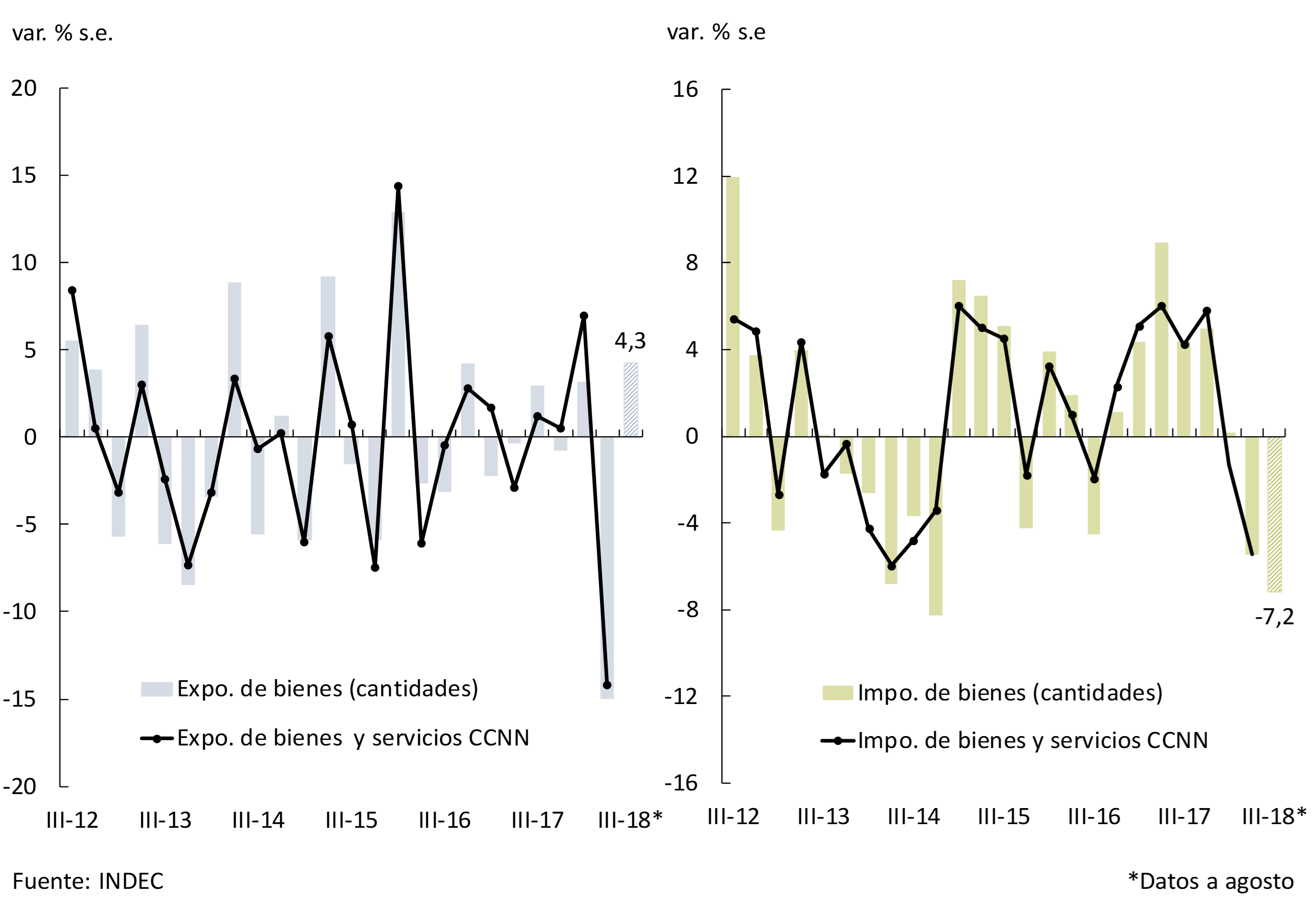
In this way, the data for the July-August two-month period confirmed the expected trends: the quantities exported of goods increased 4.3% s.e. in relation to the previous quarter and those imported fell 7.2% s.e. with falls in all uses, with purchases associated with investment being more noticeable. On the services side, similar behaviour is expected, highlighting the rebound in inbound tourism and a marked decrease in outbound tourism. In particular, in the month of August, the number of foreign tourists who entered the country by air increased 7.4% YoY, while the departure abroad of Argentine tourists by the same route decreased by 11.9% YoY.
Figure 3.8 | Exports and imports of goods and services
For the third quarter, the BCRA expects total exports and imports to follow a similar trajectory to that observed up to August in goods (see Chart 3.8), so that the contribution of net exports to quarterly output growth in the third quarter will be positive, close to 3 p.p.
Box. La reducción prevista del déficit de cuenta corriente
In the last four quarters to the second quarter of 2018, Argentina accumulated a current account deficit equivalent to 5.6% of GDP. As mentioned in the April 2018 IPOM, this was mainly due to the negative gap between savings and investment in the public sector. In the absence of a deep domestic capital market, the government’s strategy of gradual reduction of the fiscal deficit implied high external financing needs. Dependence on savings from the rest of the world was thus one of the main vulnerabilities of the economy.
The risk of illiquidity associated with this strategy materialized after a series of external and internal shocks that affected the local economy, which caused a change in market sentiment that manifested itself in a sharp depreciation of the peso and a reduction in the demand for domestic assets (both residents and non-residents). As a result, the multilateral real exchange rate has risen 38% so far this year and is at levels similar to those of the second half of 2010. Economic activity was affected by the sudden change in relative prices and entered a recessionary phase from the second quarter of 2018.
The real depreciation of the peso and lower domestic absorption are expected to contribute to a significant adjustment of the external imbalance starting in the third quarter of 2018. Imports are expected to be influenced by the negative “income effect” linked to the lower level of economic activity. There is also empirical evidence indicating that a large change in relative prices causes a “substitution effect” in spending patterns in favor of domestic goods14 and limits the purchase of foreign goods. The outlook on how the current account deficit will be reduced still bears characteristic features of the typical adjustments that the Argentine economy has historically experienced: a preponderance of the income effect over the substitution effect. In the future, and as the floating exchange rate regime is consolidated, external adjustments are expected to be softer (see Section 1 / Exchange rate float and volatility of the IPOM current account of October 2017).
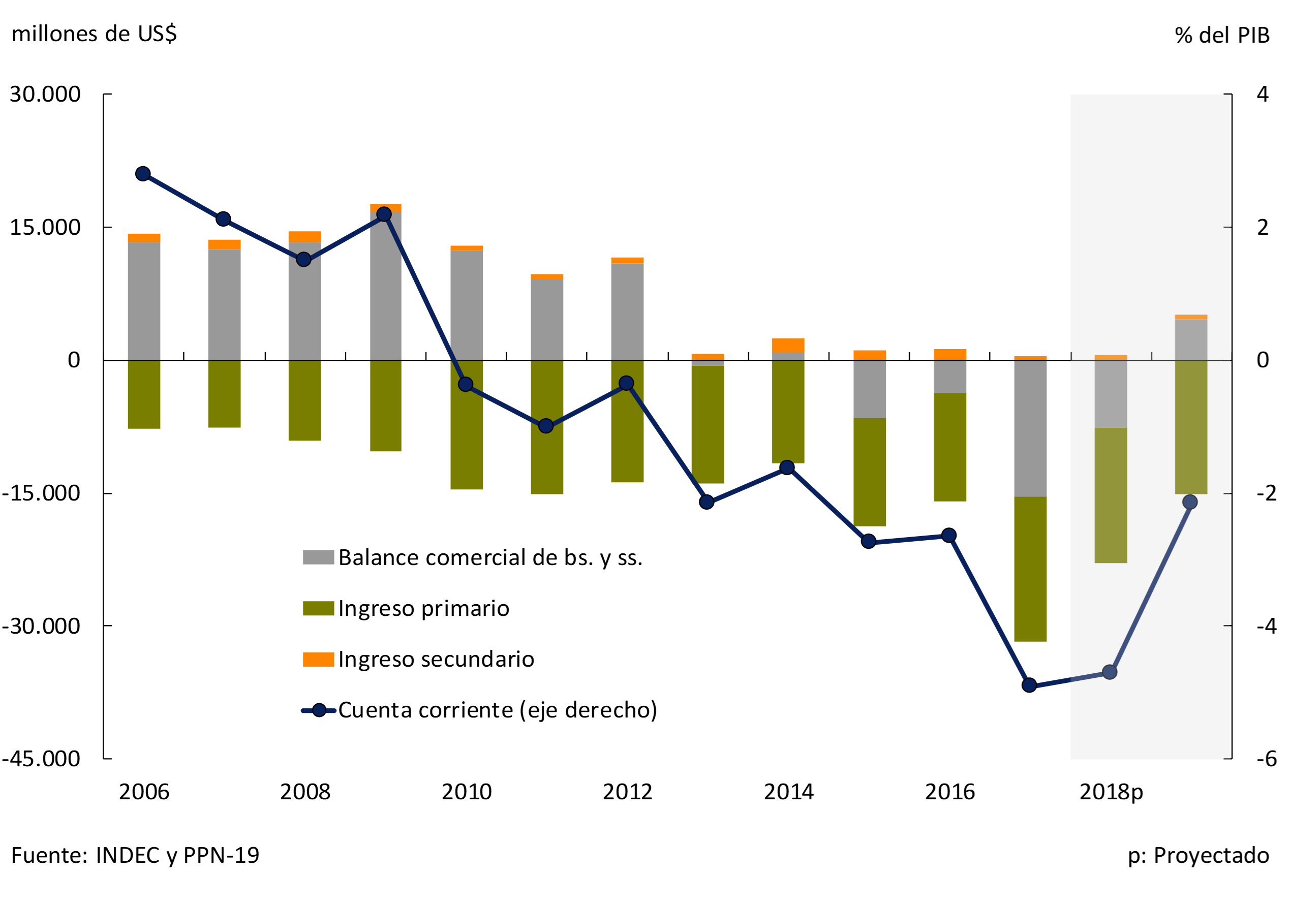
Indeed, the first signs that the economy is on track to reduce its current account deficit have already begun to emerge. In June, both the quantities imported of goods and the departures of resident tourists by air fell 11% y.o.y. and 3% y.o.y. respectively, and thus stopped a streak of uninterrupted increases during the previous 15 months. In the third quarter, both variables showed declines again. The prolonged stress in the financial markets and the deterioration in the outlook for economic growth will imply that external adjustment will accelerate relative to what was anticipated in the July IPOM (see Figure 3.9).
Figure 3.9 | Current account of the balance of payments
On the other hand, as mentioned in the July IPOM, the expected harvest for the following season is among the highest in history, which would imply a marked increase in agricultural exports in 2019 (in particular of the soybean complex) in relation to the low base of comparison of 2018. Likewise, the new path of fiscal consolidation foreseen, more demanding than the previous one, will imply a faster closing of the savings-investment gap in the public sector, which is —as mentioned— one of the main determinants of the current account deficit (see Section 2 / Fiscal consolidation and IPOM current account result of July 2018).
The confluence of the effects of substitution (of foreign goods by domestic goods) and income (caused in the short term by the recession), added to the higher agricultural exportable balances, would allow a reversal of the trade balance of goods (from a deficit situation in 2018 to a projected surplus for 2019) and a significant reduction in the deficit of services. This would allow Argentina to considerably moderate its current account deficit in 2019 and thus reduce one of its main vulnerabilities.
3.1.3 The fall in economic activity was disseminated at the sectoral level
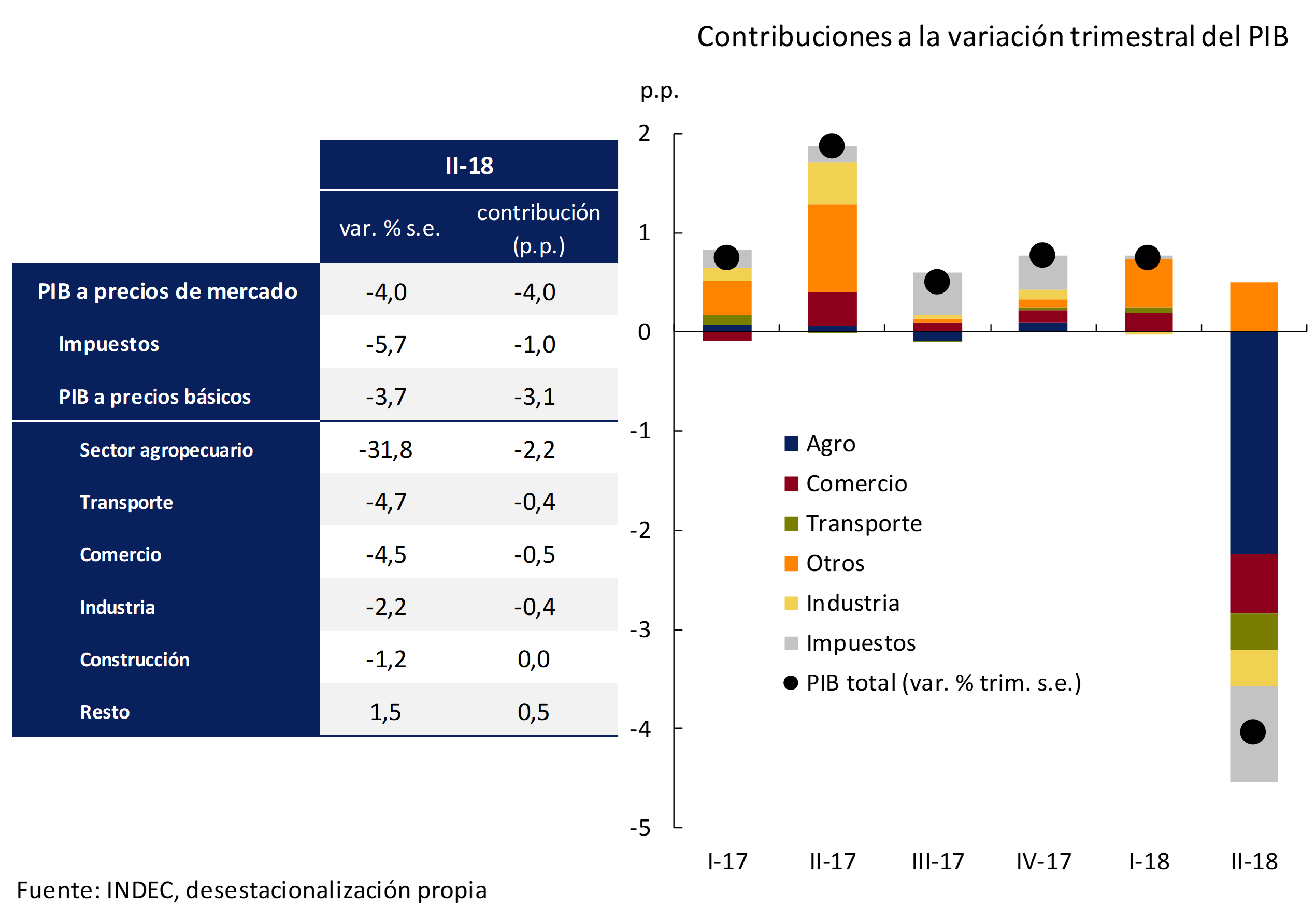
During the second quarter, the aforementioned fall in domestic demand and the negative impact of the drought explained the sharp contraction in GDP, which was widely publicized: 14 of the 20 sectors of activity fell compared to the first quarter. The fall in total output15 was a combination of a performance of the agricultural sector contemplated in the adverse scenario of the previous IPOM and a contraction of the rest of the sectors in line with the expected central scenario (-3.7% s.e. observed vs. -3.5% of the scenario; see Table 3.1, IPOM July 2018). GDP measured at market prices fell 4% quarter-on-quarter. This difference is explained by a sharp drop in tax collection (-5.7% s.e.), which is generally more volatile than GDP at basic prices and therefore tends to deepen the variations in the measurement at market prices.
Figure 3.10 | Sectoral evolution of activity
The gross value added (GVA) of the goods-producing sectors—excluding the agricultural sector—showed a fall of 1.7% s.e., essentially explained by the contraction of industry. Services fell by a similar percentage (-1.8%) due to the sharp deterioration in transport and trade, which were not only affected by the fall in domestic demand but also by the decrease in agricultural activity. The rest of the services, less linked to the economic cycle, continued to increase, although at a slower pace compared to that evidenced in the first quarter.
The fall in agricultural output during the second quarter was in line with the adverse scenario of the previous IPOM (-31.8% quarter-on-quarter vs. -30% of the scenario) with a direct impact on the variation in total GDP of -2.2 p.p. (see Figure 3.10).
In the third quarter, different indicators showed a deepening of the contraction of the non-agricultural sectors. The direct and indirect impact of the normalization of agricultural products would partially offset the contraction in the rest of the sectors.
The sharper fall in domestic demand during the third quarter had a widespread effect on the different sectors of GDP. With data up to August, the Monthly Industrial Estimator (INDEC) fell 1.6% s.e. compared to the previous quarter, the Industrial Production Index (IPI) of O.J. Ferreres contracted 1% s.e. and that of FIEL, 3% s.e., while construction was affected by the deterioration of financial conditions and the slowdown in public works and deepened its contraction from -1.2% s.e. in the second quarter to a fall of 2.3% s.e. in the second quarter. the third. 16 Services linked to the economic cycle, such as transport and trade, fell during the third quarter, at a slower rate than the rest of the non-agricultural product. The base effect compared to the second quarter (negatively influenced by the drought) offset part of the fall in these services.
Once the short-term contractionary effects of the depreciation of the local currency have been overcome, it is expected that a higher level of the real exchange rate will boost the activity of the tradable sectors (exporters and import substitutes) due to the improvement in their relative prices.
3.1.4 Labour market conditions reflected the first impacts of the contractionary phase of activity
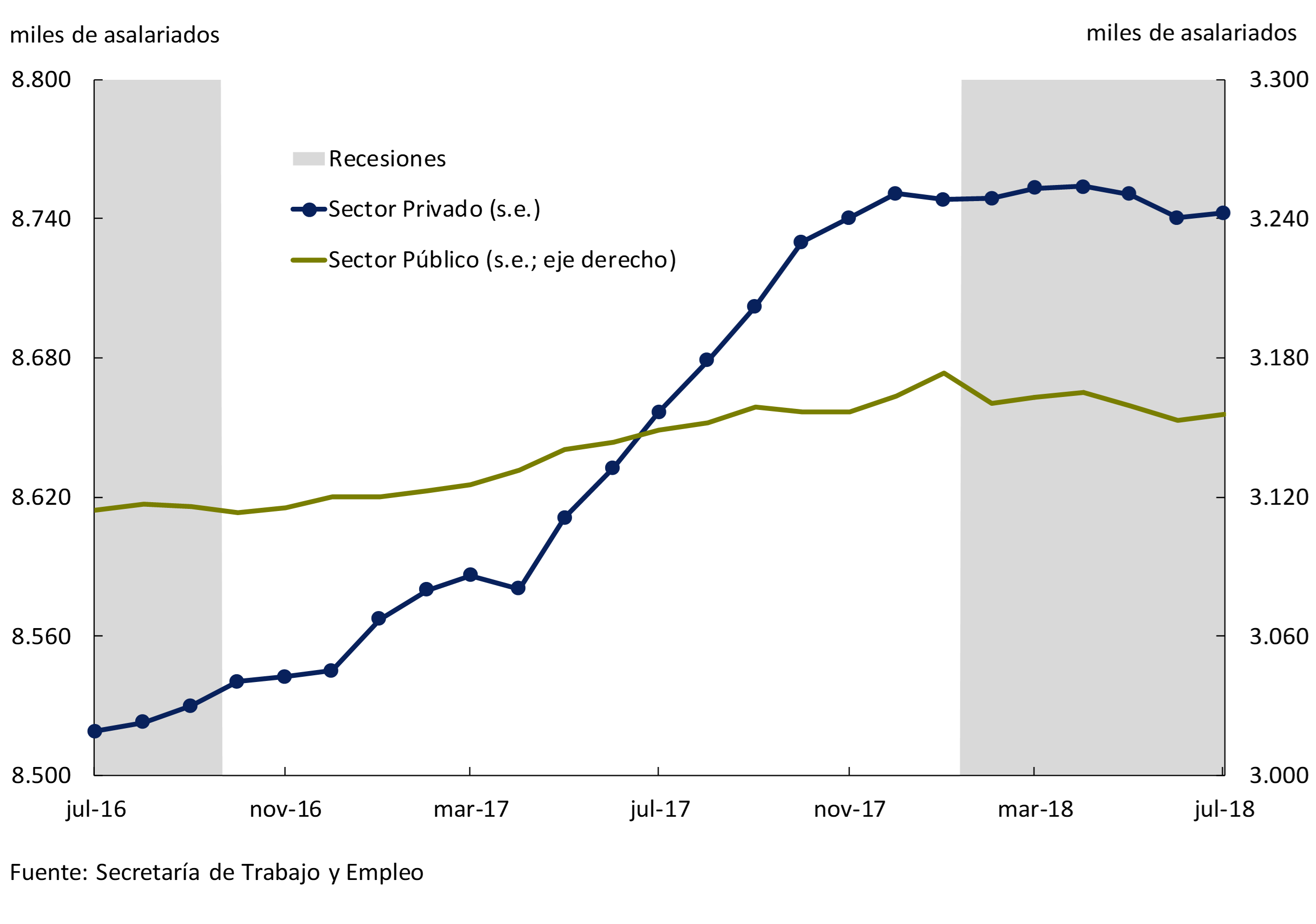
In the second quarter of 2018, the fall in GDP led to a moderate contraction in formal employment, halting the expansion cycle that began in mid-2016 (see Figure 3.11). Formal salaried work showed stagnation between December and March and then began a slight contractionary trend.
Figure 3.11 | Registered employment (excluding the social monotax)
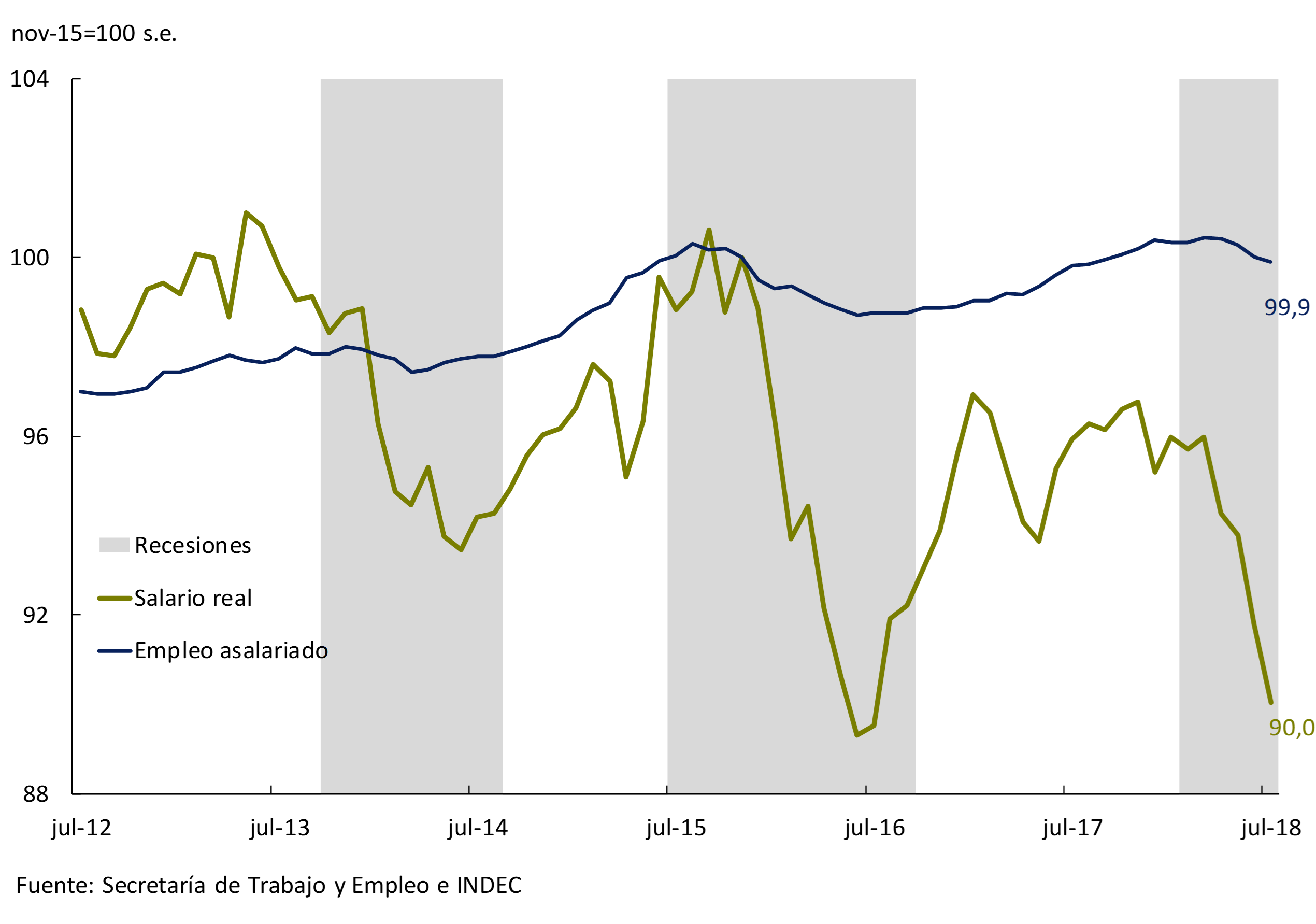
This dynamic was foreseeable in the initial part of a contractionary phase. As in other recessions, firms often choose to reduce the rate of staff17, to underutilize the labor factor through suspensions and reductions in hours worked, and/or to delay the adjustment of nominal wages before deciding on a plant cut (see Figure 3.12). This dynamic is enhanced under a flexible exchange rate by allowing a greater adjustment of real wages and a lower contraction of employment.
The procyclical nature of real wages also helps to minimize job losses, containing the harmful effects that unemployment has on an economy in the long term. In the current adverse scenario, exchange rate flexibility is what facilitates absorbing the shock mainly through prices and not through layoffs.
Figure 3.12 | Real wages and salaried employment
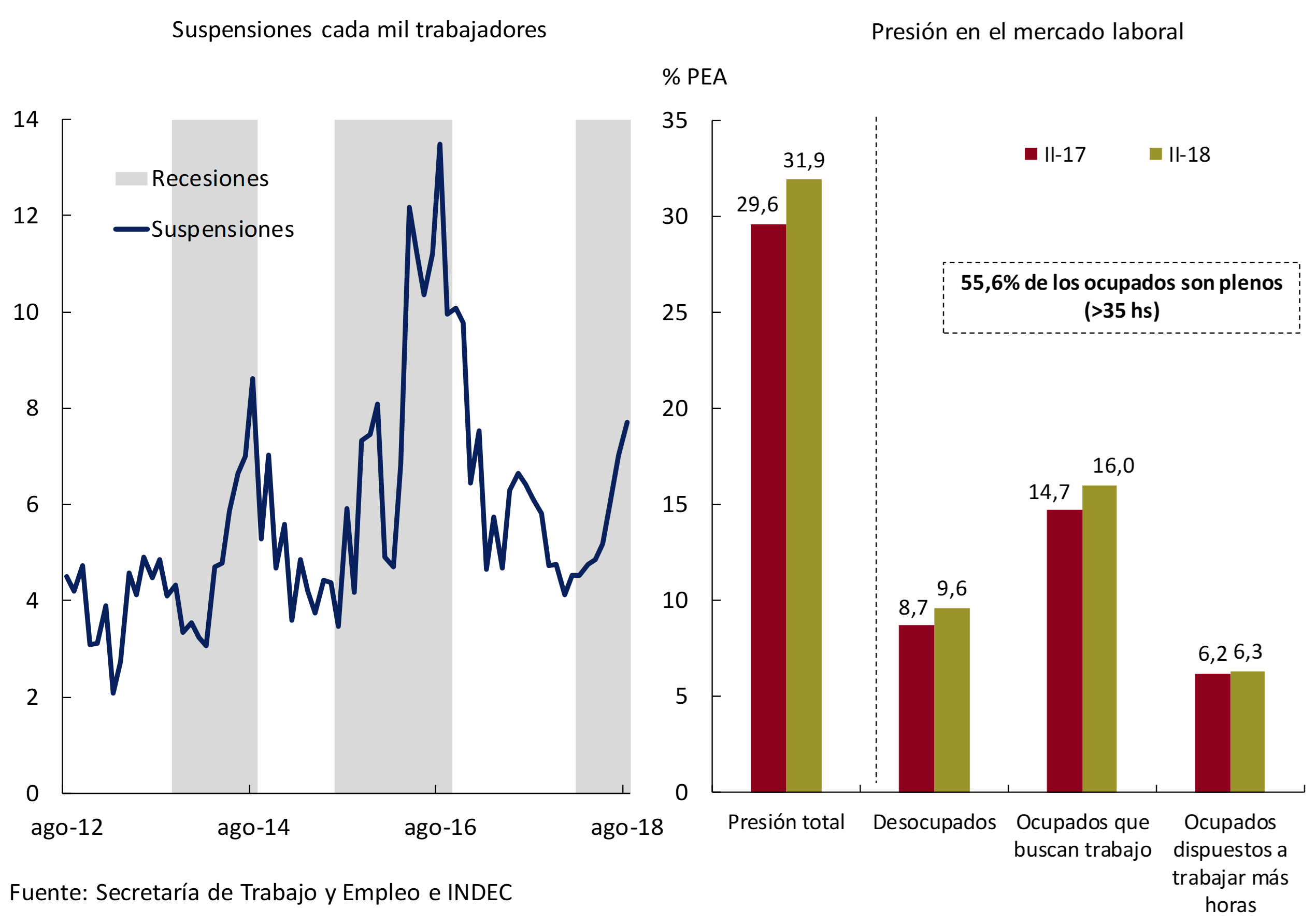
The increase in suspensions, together with the reduction in working hours and the decrease in the purchasing power of wages, was reflected in an increase in pressures in the labour market: the number of people who were inactive and decided to look for work, who were employed or underemployed and who are looking for another job and/or are willing to work longer hours, it rose from a year ago (see Figure 3.13).
Figure 3.13 | Suspensions and pressure on the labour market
Employment was most affected in the construction and industrial sectors and, to a lesser extent, services linked to the product cycle, such as transport, commerce, and hotels and restaurants. Jobs in the primary sector remained stable despite the impact of the drought on activity (see Figure 3.14).
Figure 3.14 | Formal salaried employment by sector

The growth rate of total employment continued to show positive figures in annual terms: the employment rate increased 0.4 p.p. in the second quarter (standing at 41.9%). The economy created jobs at a faster rate than population growth (2.2% YoY and 1.1% YoY, respectively). The unemployment rate grew 0.9 p.p. (to 9.6% of the EAP), explained by the growth in the number of people who joined the job search (3.2% y.o.y.) and who were unable to get a job.
The prospects for job creation for the coming months deteriorated in line with the contraction in activity in the third quarter. The Survey of Labor Indicators of the Ministry of Labor and Production for the month of August showed a reduction in net employment expectations, standing at 0.2%18 (1.4 p.p. compared to the previous month).
3.2 Outlook
The macroeconomic projections contained in the 2019 Budget Bill contemplate a fall in GDP of 2.4% in 2018 and the beginning of a recovery in 2019. This path of gradual recovery of the economy is shared by market analysts who participate in the REM and anticipate variations of -2.5%, -0.5% and 2.2% for 2018-2020 (see Figure 3.15).
Figure 3.15 | GDP Market Projections
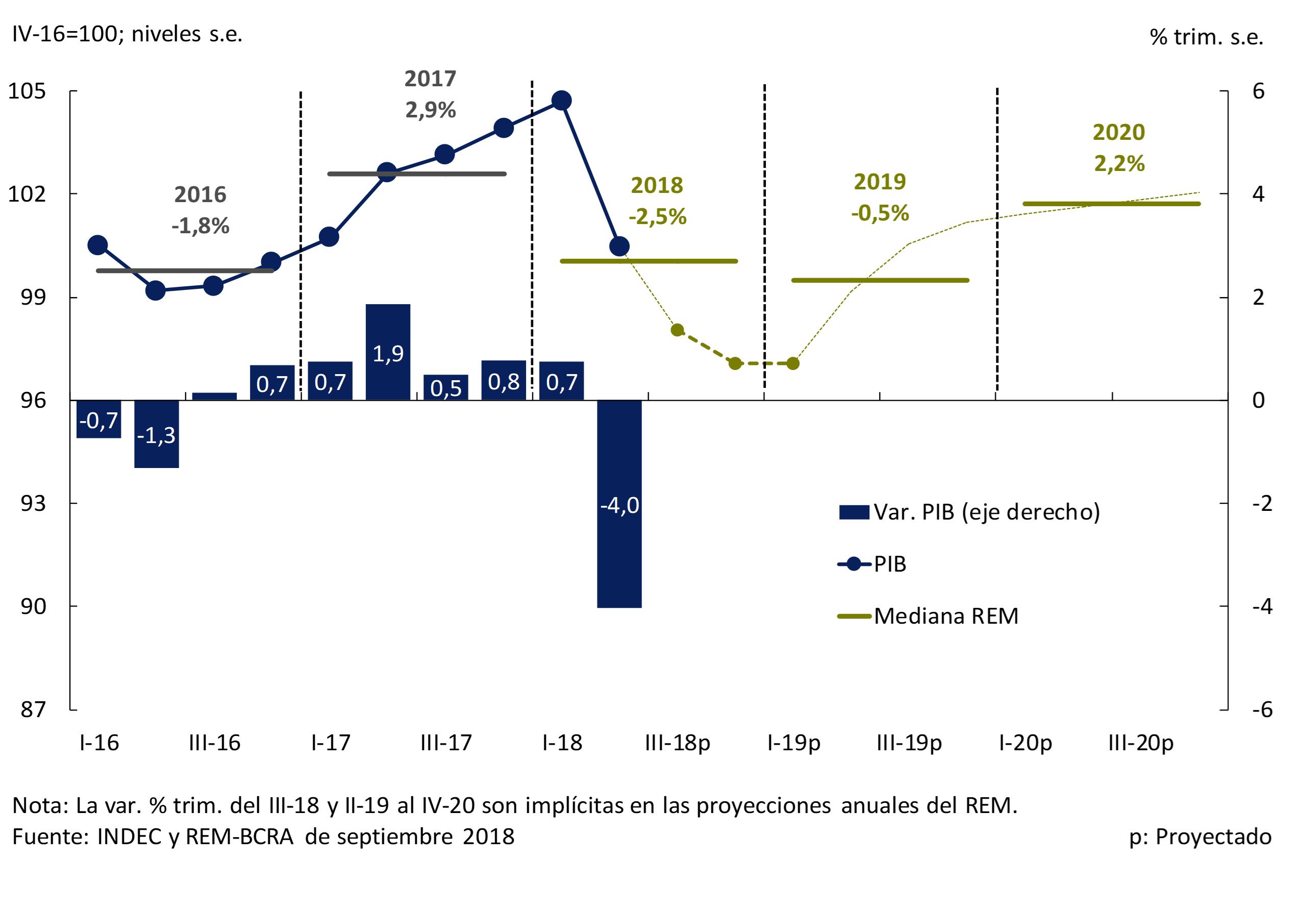
These projections are consistent with the BCRA’s base scenario, which foresees the beginning of an expansionary phase in 2019, based on the better performance of the export sector and the normalization of the functioning of the financial markets, contributing to the correction of the current account imbalance.
On the fiscal front, the broad set of measures announced by the Executive Branch in September points to a sharp reduction in the imbalance in the public accounts – with lower capital expenditures, cuts in subsidies to public service rates and other expenditures – eliminating a factor of uncertainty that will gradually reduce the cost of financing for the private sector. This will facilitate the rebalancing of growth sources towards a greater participation of the sectors that produce tradable goods and services.
The energy sector will continue to show a great performance because its investment and expansion plans were not affected by the change in market conditions. The expected increase in oil and gas production over the next few years will make it possible to reduce the external deficit (see Section 1. Advances in the energy sector). For 2019, investments through the PPP system are expected for more than 16,000 million pesos, according to data from the 2019 National Budget Bill. These projects will be aimed at expanding and improving the efficiency of the energy matrix19.
There are also good prospects for agricultural production, with soybean and corn harvests expected to reach at least the levels of the 2016/2017 season, which means increases of approximately 45% and 24% y.o.y., respectively, and that beef production will continue with an increasing trend20.
Exports in general will be a source of traction for the activity since, with more favorable relative prices, it is expected that in 2019 Argentina’s main trading partners will show the highest growth in the last eight years (see Chapter 2. International Context), although volatility persists in relation to the development of the international financial framework.
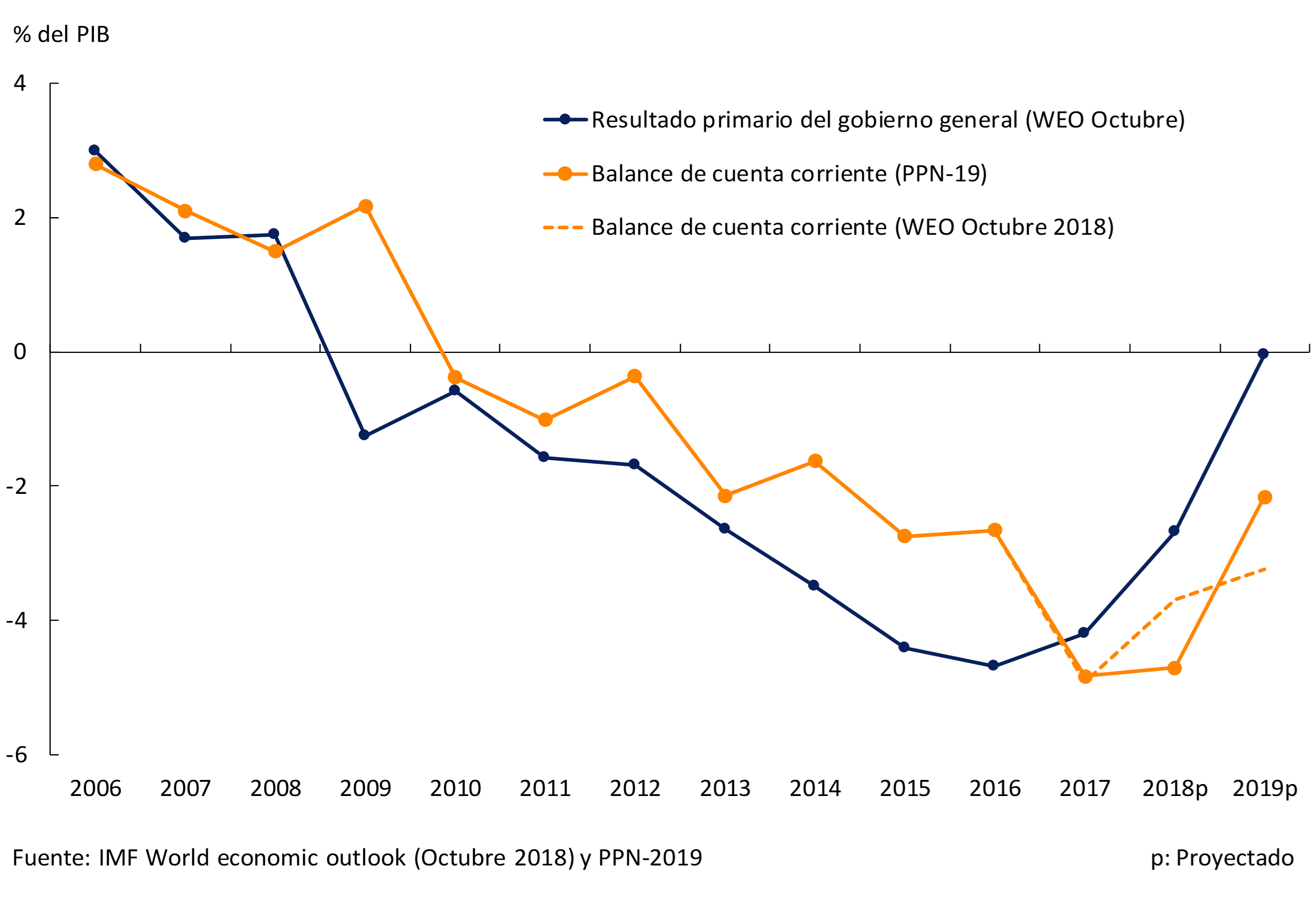
In this context, the current account projections contemplated in both the 2019 Budget Bill and the IMF estimate a marked reduction in the external deficit that will eliminate a systematic source of vulnerability and improve the sustainability of growth over time (see Figure 3.16).
Figure 3.16 | Current Account and Tax Result
4. Pricing
During the third quarter, inflation increased, standing at 4.5% monthly average. The general level mainly reflected the increase in core inflation, which gained dynamism compared to previous months, driven by a new episode of depreciation of the Argentine peso. This occurred as a result of a deterioration in global financing conditions for emerging economies that, in the case of the local economy, was accentuated by internal vulnerabilities. The new episode raised the risk of a greater unanchoring of the public’s expectations. In response, the BCRA introduced a new monetary policy framework based on strict control of the monetary base. The new regime pursues the objective of recovering the nominal anchor for inflation expectations.
In the short term, inflation would continue to be high due to the transfer to prices of the rise in the nominal exchange rate observed in recent months and due to pending adjustments in relative prices in some public services. For the rest of the year, the Market Expectations Survey anticipates a slowdown in inflation to 3% per month by December of this year. Within the framework of the new monetary policy scheme, market analysts’ expectations foresee a moderation in inflation for 2019 and 2020.
4.1 Prices continued to accelerate driven by depreciation
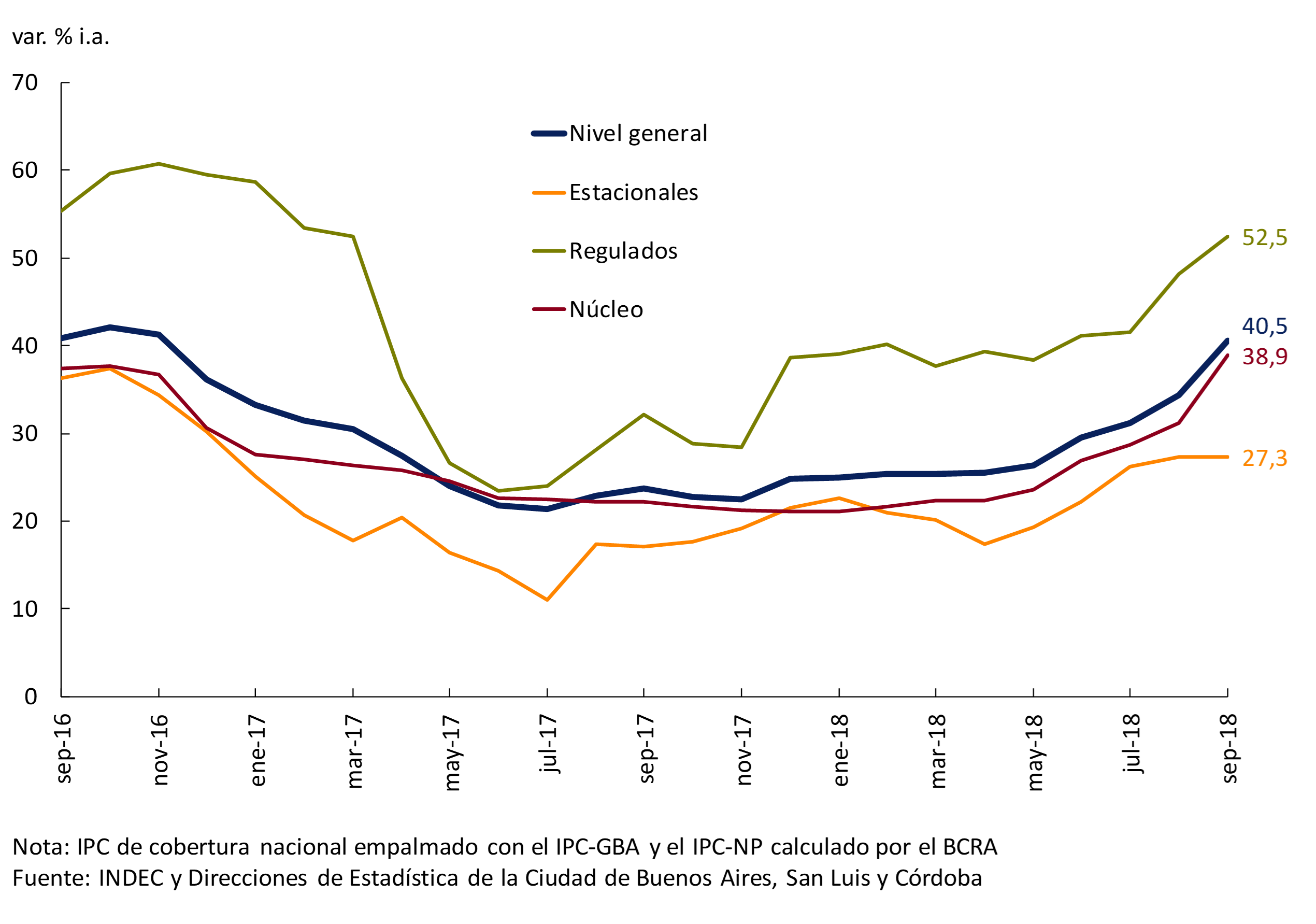
During the third quarter of the year, inflation gained momentum, reaching monthly average rates of 4.5% (see Figure 4.1). Prices accumulated a 32.4% increase in September and are 40.5% above the levels of a year ago. The factor that explains the acceleration of prices to a greater extent was the depreciation of the domestic currency.
Figure 4.1 | Inflation. General Level and Core
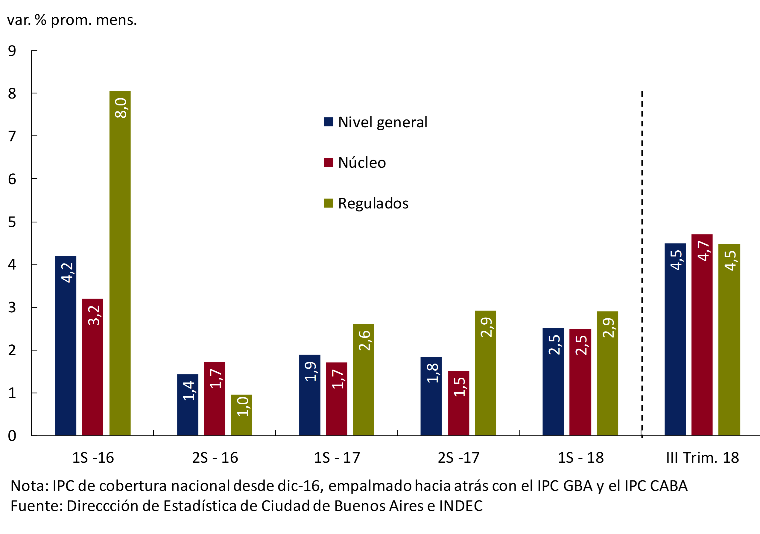
Figure 4.2 | Real Exchange Rate
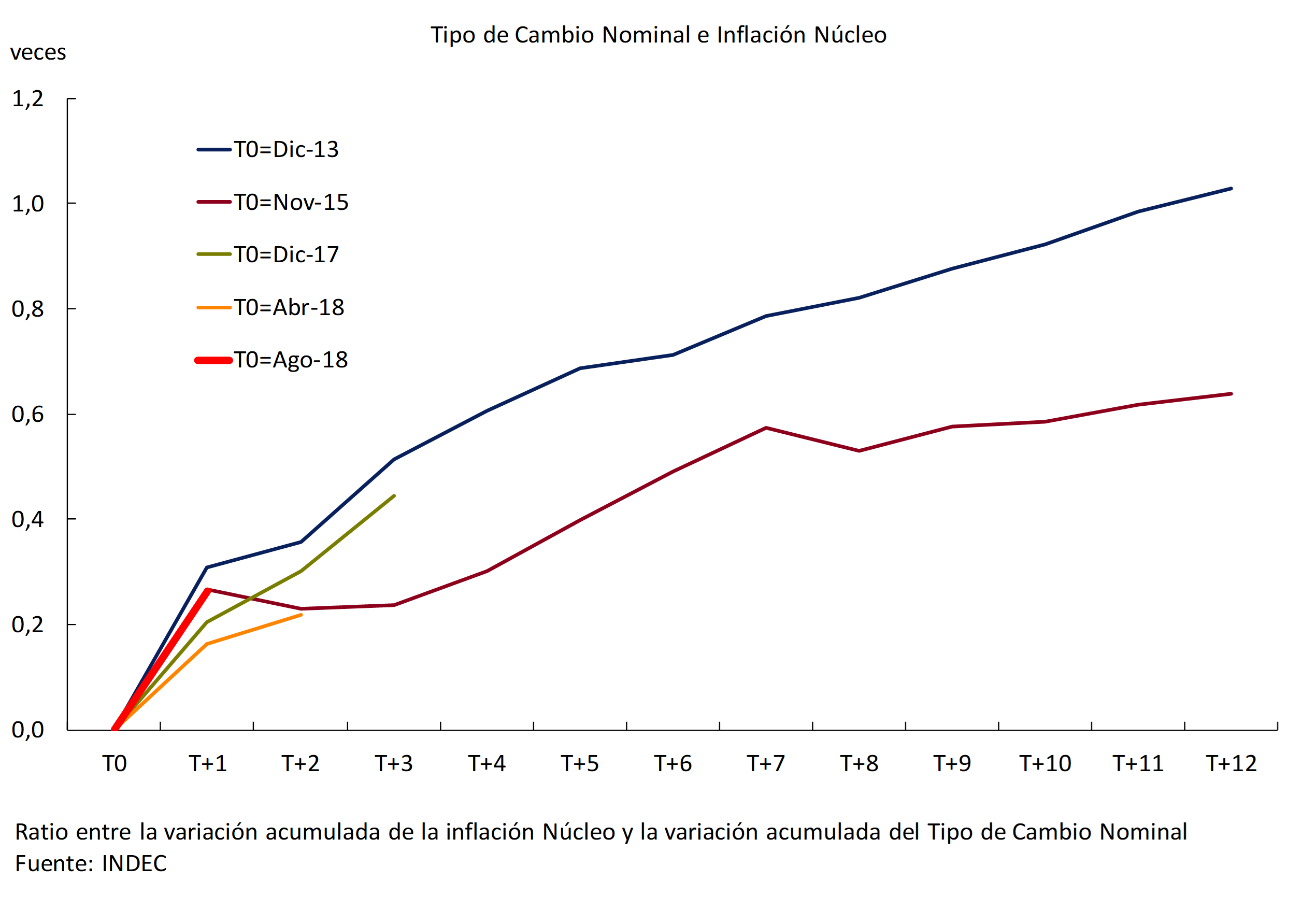
In 2018, two episodes of devaluation of the domestic currency of significant magnitude can be identified. The cumulative effect of both shocks resulted in a rise in the exchange rate considerably higher than inflation, allowing the real exchange rate to depreciate to levels similar to those of 2007 (see Figure 4.2). In the first episode, the bilateral nominal exchange rate with the dollar registered a 35% increase, which occurred gradually between mid-April and mid-June. The second corresponds to a discrete increase in the exchange rate at the end of August (approximately 30% depreciation). Although these increases are similar in the magnitude of the increase, they had differential effects on prices (see Figure 4.3). The second episode deepened uncertainty, led to a further price correction and raised the risk of a further unanchoring of inflationary expectations. In order to reduce uncertainty and recover the anchor above expectations, the BCRA modified its monetary policy scheme. The new regime contemplates a goal of zero growth of the monetary base until mid-2019 (see Chapter 5. Monetary Policy).
Figure 4.3 | Core Inflation and Nominal Exchange Rate
Core inflation continued to gain dynamism and was the one that had the greatest impact on the acceleration of the general price level. Thus, in the third quarter this measurement of inflation (which excludes regulated and seasonal inflation) averaged increases of 4.7% monthly, 1.8 p.p. above the average rate of the previous period. In September, this component marked a rate of change of 7.6% (the highest since April 2002), accumulating an increase of 33.1% so far this year and a year-on-year increase of 38.9% (see Figure 4.4).
Figure 4.4 | Inflation. Year-on-year growth
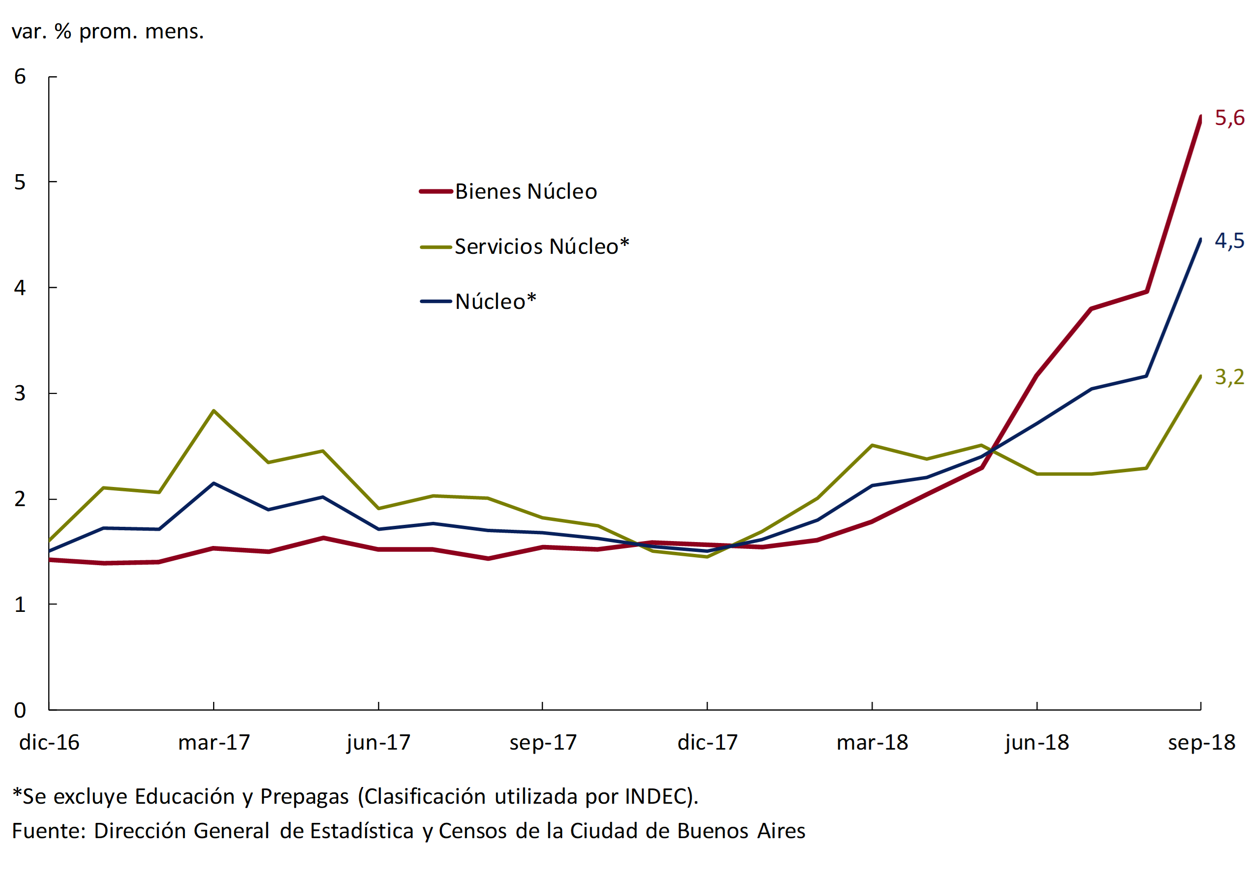
Goods included in core inflation, particularly food, were the biggest drivers of the acceleration over the past two quarters (see Figure 4.5). Because of their tradable nature, these products are more sensitive to currency depreciation. Meanwhile, private services showed more limited increases in the period. In addition, both goods and services were indirectly influenced by increases in public services.
Figure 4.5 | Core inflation. Opening for Goods and Services (mobile avg. 3 months)
Regulated goods and services also contributed to the acceleration of inflation. In the third quarter they increased at a similar rate to that of core inflation, although in the year they accumulate a higher increase. The most significant increases were verified in the prices of fuel for cars, public transport and electricity. Gasoline, whose prices are deregulated, registered increases above inflation. Fuels were influenced by the depreciation of the peso and the scheduled increase in internal taxes. In mid-August, a new price adjustment scheme staggered over three months came into force for buses and trains in the GBA. This last scheme implies a total increase of 35% and complementary to the increases of the first semester. Thus, in the year they accumulate increases of 92% for buses and 74% for trains. With regard to electricity, in the eighth month of the year, new rates began to apply that correspond to the semi-annual update of this service. In year-on-year terms, regulated goods and services reached growth rates close to 51.7% y.o.y.
Wholesale prices, on the other hand, saw higher increases than those of consumer prices, averaging a monthly increase of 8.4% in the third quarter (+3.2 p.p. above the average monthly increase of the second quarter of 2018). This behavior is explained by the high contemporary correlation between wholesale prices, its basket is almost exclusively composed of goods, and the Nominal Exchange Rate. Wholesale indices and the goods that make up the consumer basket are the ones that reacted the most to the depreciation of the peso, given their nature as tradable goods21 (see Figure 4.6).
Figure 4.6 | Wholesale Prices and Nominal Exchange Rate

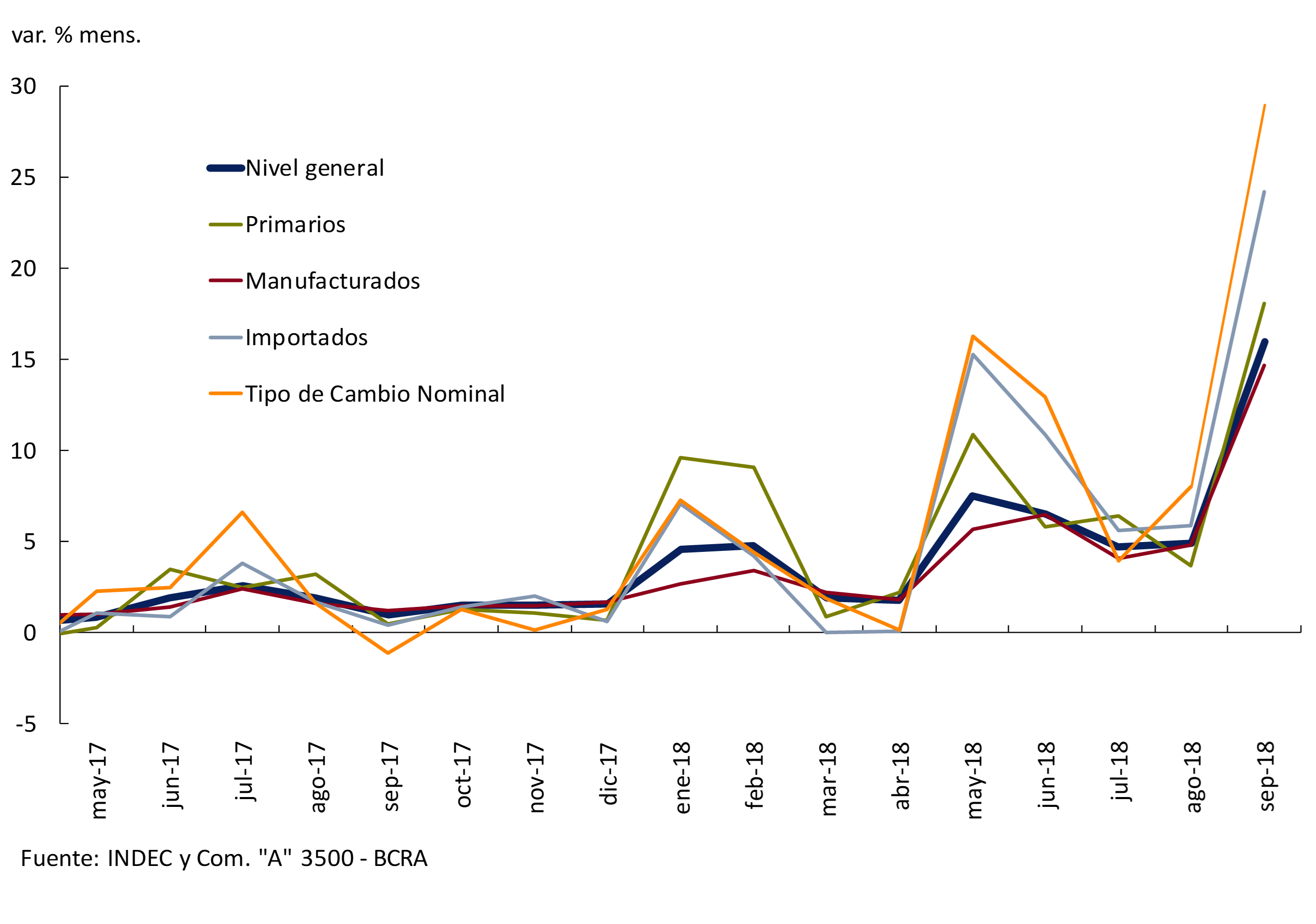
The acceleration of the IPIM in the third quarter of the year was mainly due to the dynamics of the prices of manufactured products (see Figure 4.7). The increases that had the greatest impact on the rise in manufacturing prices were: Chemical substances and products, Refined petroleum products, Food and beverages, Motor vehicles and Machinery and equipment. New increases were added to agricultural products in pesos, on which the depreciation of the local currency played a determining role. The crude oil and gas component also averaged high increases in the period basically due to the increase in crude oil (monthly average of 2% in dollars), which was boosted by the depreciation of the peso. The prices of imported products were once again the ones that increased the most, directly affected by the dynamics of the exchange rate. It should be noted that this component has a limited impact on the general level of the IPIM, due to its low weighting. The monthly acceleration of wholesale prices during the third quarter of the year boosted the year-on-year rates of change, which rose to values close to 60% in the third quarter of 2018.
Figure 4.7 | IPIM by components
4.2 Wage patterns continued to show limited variations
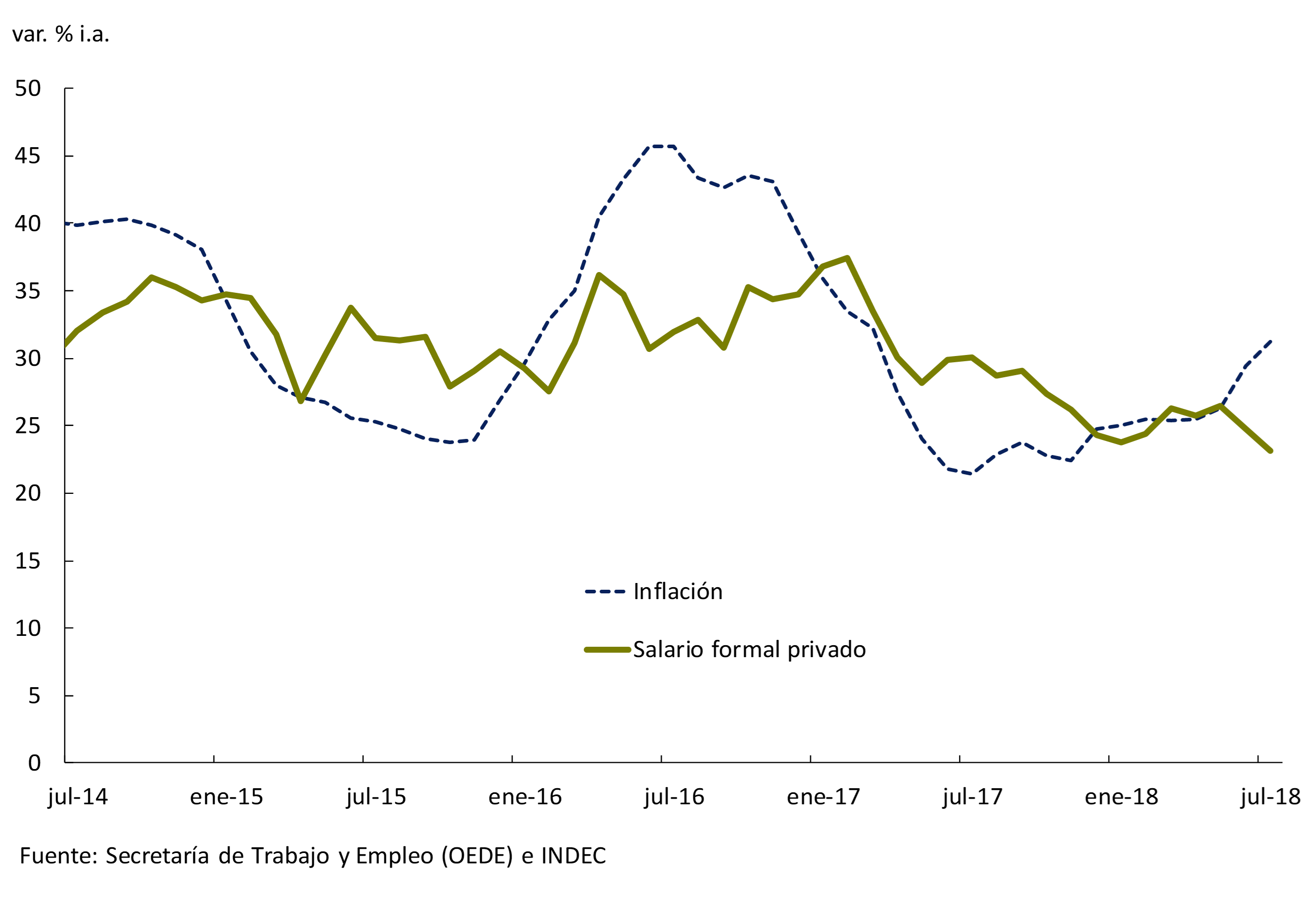
In the middle of the year, nominal wages in the formal private sector showed a variation compared to 2017 of around 25% according to data from the Ministry of Labor and Employment. Most of the parity negotiations corresponding to 2018 reflected a nominal increase in remuneration of 25.6% y.o.y. in the second quarter, 5 p.p. below the figures of a year ago. By the third quarter of the year, wages would grow at a similar rate. For the last part of the year, an acceleration in the nominal increase in remuneration is expected as a result of the update of tranches, readjustment clauses and extraordinary increases, to compensate for the acceleration in prices. However, wages would end the year with a lower year-on-year rate of change than retail prices (see Figure 4.8).
Figure 4.8 | Evolution of the nominal wage
The salary guidelines for 2019 would include some retroactive adjustment as compensation in the first quarter, to then align with market inflation expectations. In any case, the salary negotiations of each sector will be conditioned by its economic situation and prospects.
4.3 Market analysts’ expectations revised upwards in a context of greater dispersion in projections
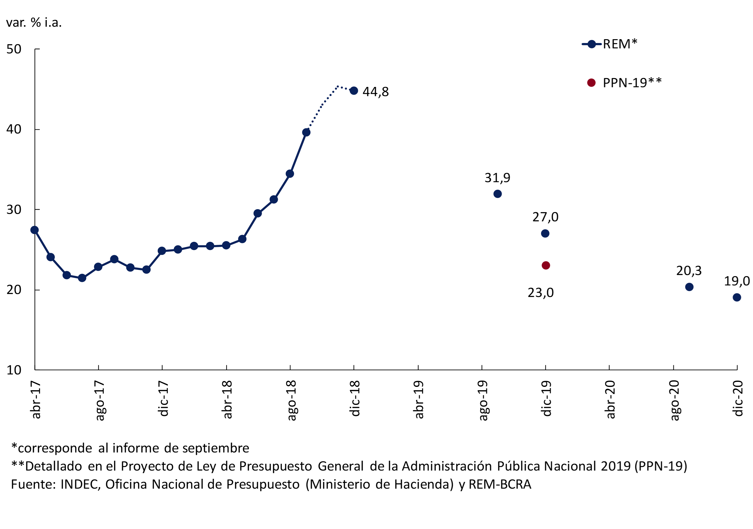
For the last quarter of the year, the Market Expectations Survey anticipates a gradual slowdown in monthly inflation rates. In December, according to the REM, consumer prices would grow at a rate close to 3% (see Figure 4.9). Given this trajectory, the year would end with inflation of 44.8% y.o.y., which implies a revision of 14.8 p.p. upwards compared to what was published in the previous IPOM.
Figure 4.9 | REM analysts’ monthly inflation expectations*
Within the framework of the new monetary policy scheme, which contemplates a quantitative target on the monetary base22, the expectations of market analysts participating in the REM foresee a moderation of inflation in the short and medium term.
In line with the REM, the BCRA also forecasts a gradual reduction in inflation for the coming months. This is because some factors would continue to put upward pressure on prices. On the one hand, the strong depreciation of the peso will continue to be transferred to prices, particularly of tradable goods. On the other hand, there are pending adjustments of relative prices that would materialize in the short term.
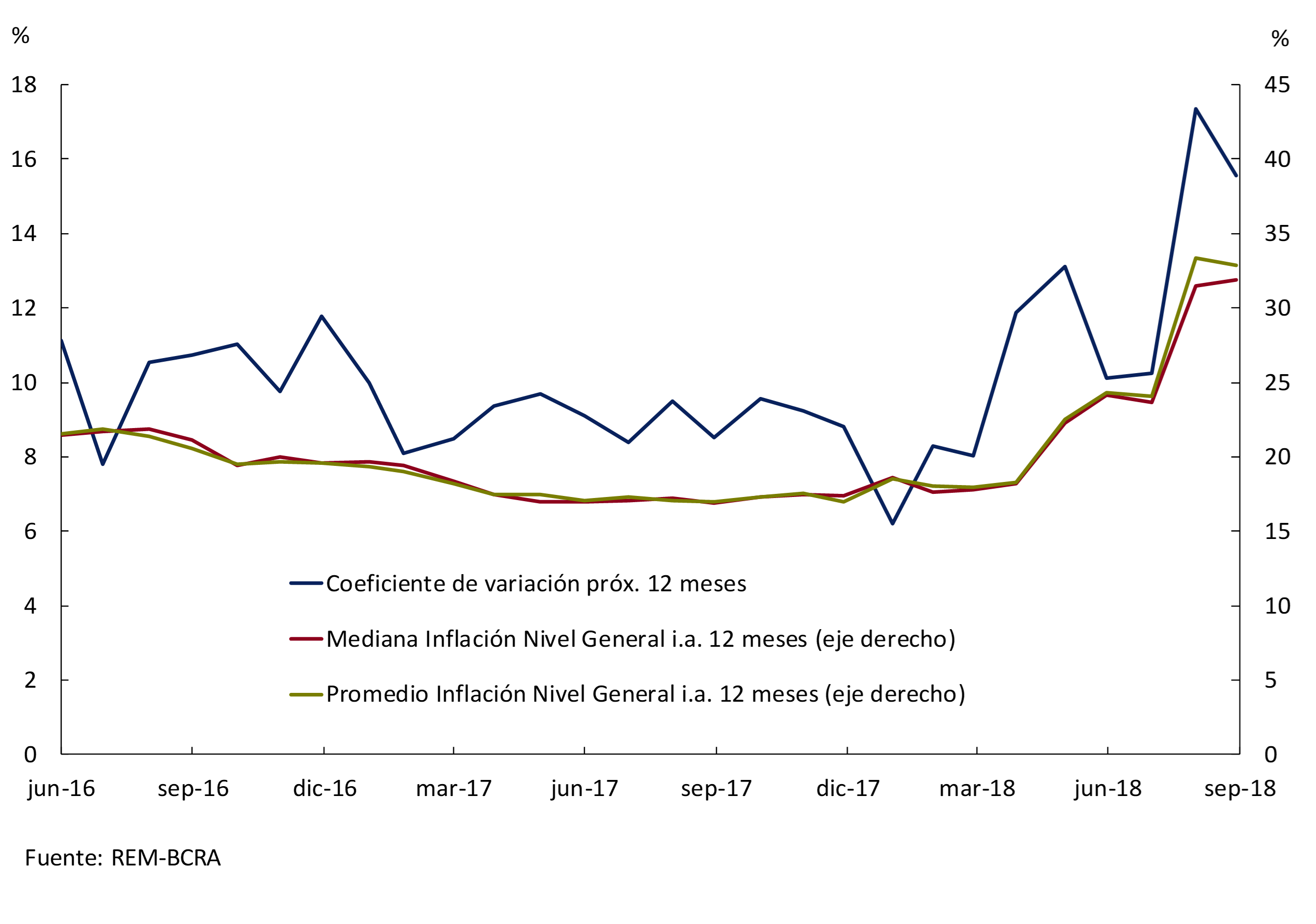
For the next 12 months, the average of the projections of REM analysts anticipates a price variation of 32.9%, showing a slight decrease of 0.5 p.p. compared to the previous survey. Since January 2018, higher 12-month expected inflation has been associated with greater uncertainty around future inflation developments. The coefficient of variation23 of the responses shows an upward trend since January (a sign of an eventual unanchoring of expectations), although it showed a fall in the last record (see Figure 4.10).
Figure 4.10 | Inflation expectations for the next 12 months
The different inflation projections for the next two years show a slowdown. The estimates of REM market analysts anticipate a rise of 27% YoY for 2019 and 19% for 2020. For its part, the National Budget Bill contemplates a 23% increase in prices by the end of next year. Finally, the IMF anticipates in the World Economic Outlook (WEO) inflation of 20.2%, for the same period.
Figure 4.11 | REM inflation expectations 2018-2020
5. Monetary policy
During August, exchange rate tensions returned as a result of the confluence, again, of external and internal factors. Faced with this situation, the Central Bank took a series of measures to mitigate the pressures on the foreign exchange market and its effects on inflation: increases in the reference interest rate, interventions in the foreign exchange market, increases in legal reserves, gradual reduction of the weight of LEBACs and end of transfers to the Treasury for transitory advances and remittance of profits.
However, given the dynamics that the exchange rate was taking and its pass-through to the inflation rate towards the end of September, there was a risk of further unanchoring of inflation expectations. That is why as of October 1, within the framework of a new agreement with the IMF, the Central Bank decided to implement a new monetary policy scheme based on a monetary base target complemented by the definition of foreign exchange intervention and non-intervention zones.
In this way, the inflation targeting scheme that had been applied since September 2016 was set aside. This regime is widely used in the world, both by developed and emerging countries, and has allowed them to live with low inflation rates. However, in our country its application was hindered by the conditions presented by the economy at the beginning of its implementation: high and persistent inflation, a pending adjustment of relative prices (exchange rate and public service tariffs) and a high deficit of the public accounts financed in part with transfers from the Central Bank. Added to this was the demanding disinflation trajectory defined from the end of 2015.
Thus, with the aim of establishing a more concrete and powerful commitment to price stability in the short term that would be easily verifiable by the public, the goal of not increasing the level of the monetary base until June 2019 was established as a nominal anchor. This monetary aggregate was chosen because it is the one under the direct control of the BCRA. The goal of zero nominal monthly growth of the monetary base was defined on the monthly average of daily balances, and is adjusted with the seasonality of the months of December and June, when the demand for money increases. When a target is established on the quantity of money, the reference interest rate (the LELIQ rate) is determined by the supply and demand of liquidity, and is placed at the level that is consistent with the commitment to zero growth of the monetary base. Operationally, the monetary target is implemented through daily auctions of Liquidity Bills (LELIQ) with banks.
Recognizing the benefits of exchange rate flexibility does not imply ignoring the fact that excessive volatility of the exchange rate can be problematic, especially in our country, where the exchange rate plays a key role in the formation of inflation expectations, has a significant influence on the public’s portfolio decisions and can generate episodes of strong uncertainty that negatively affect the level of activity in the economy. That is why the monetary target is complemented by the definition of areas of intervention and non-exchange intervention. The non-intervention zone is initially defined between $34 and $44, within which the peso floats freely, and is adjusted daily at a rate of 3% per month until the end of the year.
The implementation of the new monetary regime as of October restored calm to the foreign exchange market, achieving an appreciation of the peso in the first days of operation within the non-intervention zone, along with a rise in the interest rate and a stable evolution of the LELIQ stock. At the same time, the average of the daily balances of the monetary base in the first three weeks of October was below the target for the month.
Although inflation expectations, measured in the Market Expectations Survey (REM) carried out by the Central Bank, have grown since the beginning of the exchange rate turbulence and are at high levels, it is noteworthy that the market continues to expect a slowdown in inflation at 12 and 18 months, also considering that the last survey corresponding to September was after the announcement of the new monetary scheme. In this context, it is expected that the monetary contraction generated by the new monetary policy scheme, together with the confirmation of the downward path of the primary result and the commitment assumed not to finance the Treasury anymore, will begin to be reflected in a fall in inflation expectations and the inflation rate in the coming months.
5.1 New episode of financial turbulence in August – September and the response of monetary and exchange rate policy
5.1.1 Exchange rate tensions reappeared in August
During August, exchange rate tensions returned as a result of the confluence, once again, of both external and internal factors, which found the economy still exposed to the abrupt reversal in capital flows. On the external front, financial instability from Turkey was highlighted, which produced a contagion effect on most emerging currencies (see Section 2). At the domestic level, doubts about the sustainability of the path of fiscal convergence and the financial program announced in the first agreement with the IMF and the uncertainty generated by the judicial investigations of corruption cases were relevant factors of instability24.
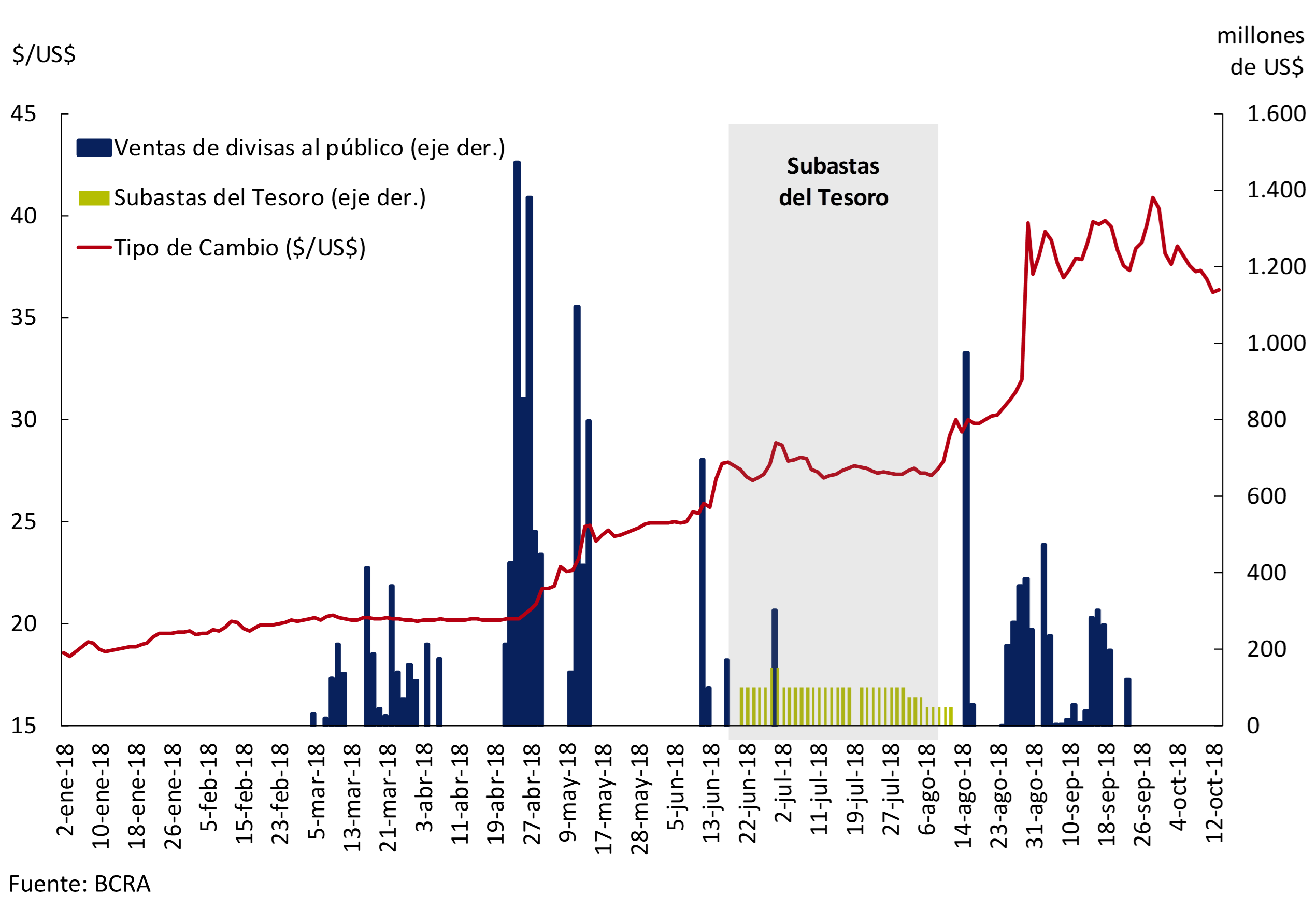
The financial turbulence intensified at the end of August, registering on the 30th an increase in the exchange rate of 24%, which then stabilized around $38.5 per dollar during September to settle at $40 per dollar towards the end of the month. Thus, the price of the U.S. currency accumulated a 42% increase between the end of June and the end of September (see Chart 5.1).
Figure 5.1 | Exchange rate, BCRA foreign exchange interventions and Treasury foreign exchange auctions
5.1.2 The Monetary Policy Response and the New Arrangement with the IMF
The Central Bank’s response to contain the exchange rate turbulence was concentrated on several fronts. On the one hand, a series of increases in the monetary policy interest rate were decided, which went from 40% per year to 45% per year on August 13 and then to 60% per year on August 30 (see Figure 5.2). At the same time, the Central Bank made foreign exchange sales to the private sector to moderate exchange rate volatility in the amount of US$ 4,532 million during the months of August and September (see Figure 5.1).
At the same time, in order to complement the contractionary bias of interest rate decisions with a more attentive monitoring of monetary aggregates, successive increases were ordered in the minimum cash requirements of deposits in pesos, both demand and time, with various integration modalities. These increases were given on August 16 by 3 p.p. for financial institutions with greater assets (integrable with pesos), on August 30 by 5 p.p. for the same group of entities effective as of September (integrated with pesos, LELIQ or NOBAC) and on September 14, effective as of 19 of that month. by 5 p.p. for banks that have at least 1% of private deposits (integrable with pesos for demand deposits and with LELIQ or NOBAC for fixed-term deposits)25.
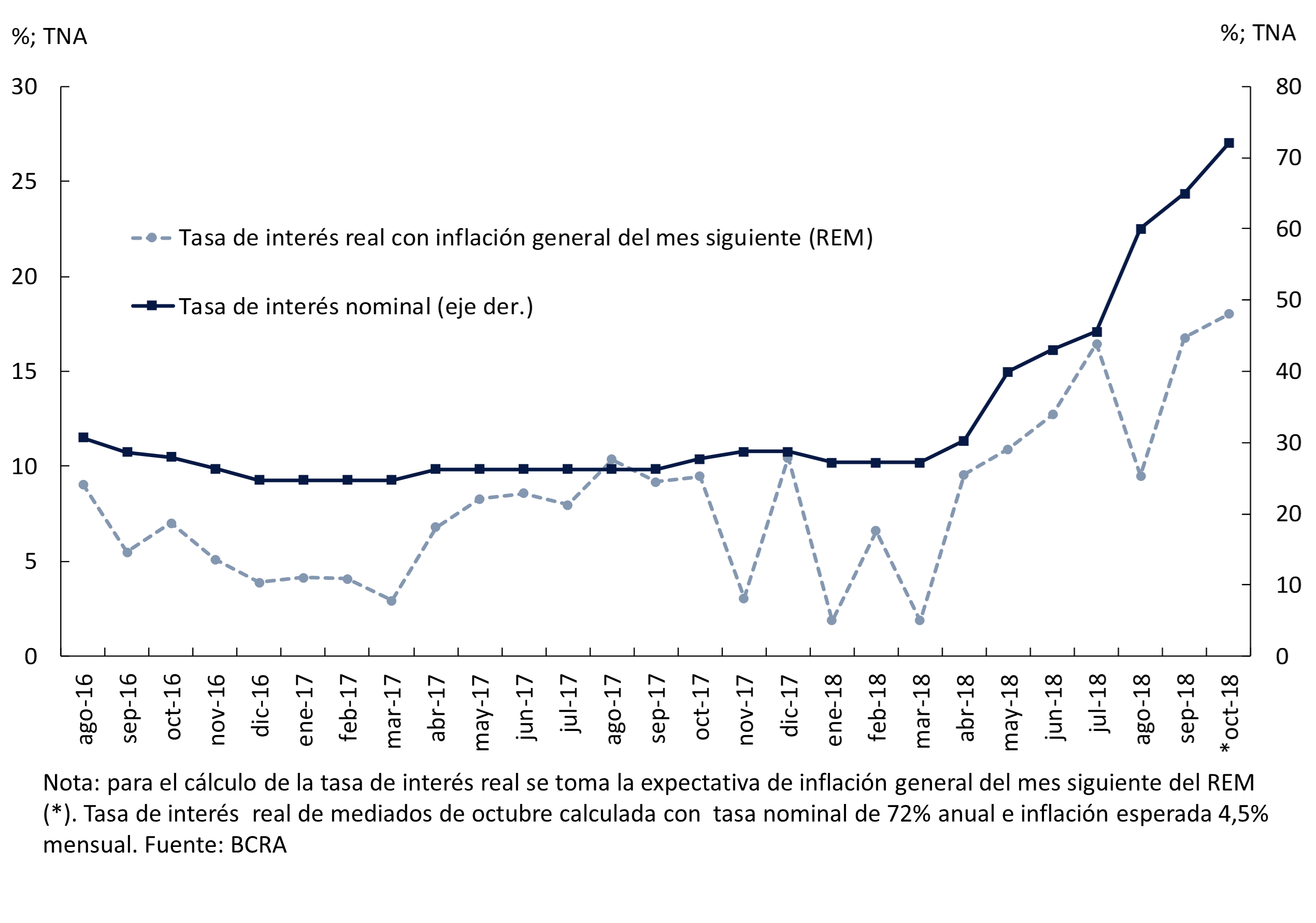
Figure 5.2 | Reference interest rate (nominal and real)26
On the other hand, in mid-August a program to cancel LEBAC was announced, with the aim of eliminating a source of instability that was at the center of the scene in the exchange rate turbulence that began in April. This stock had been formed as a result of the sterilization of fiscal deficits until December 10, 2015, the sterilization of monetary surpluses from exchange restrictions and losses from sales of dollar futures contracts prior to December 10, 2015, and the acquisition of international reserves by the monetary authority as of December 10, 2015. reaching around one trillion pesos in mid-August. To implement this reduction, it was established that in each auction the Central Bank would offer LEBAC to non-banking entities for an amount less than the maturity amount, while to banking entities it would only offer NOBAC for 1 year and LELIQ for the total maturity (the latter are instruments that can only be acquired and negotiated by financial institutions)27. This was complemented by the holding of auctions of Treasury Bills in pesos by the Ministry of Finance on the maturity dates of LEBAC with the aim of generating an attractive investment alternative in pesos. After three auctions, the stock of LEBAC fell by $ 786,193 million to $ 190,584 million in mid-October. In return for this, the LELIQ gained ground, consolidating themselves as the main instrument of intervention of the Central Bank. Thus, total interest-bearing liabilities (net passes, LEBAC and LELIQ) fell from $1,078,553 million to $715,101 million in the same period (see Figure 5.3).
Figure 5.3 | BCRA’s interest-bearing liabilities in pesos (net passes, LEBAC and LELIQ)

Finally, during the month of September, the National Government negotiated a new agreement with the International Monetary Fund aimed at clearing up doubts about the financial program for this year and the next and ending the context of uncertainty prevailing in the domestic market. Thus, the agreement reached with the technical team of the multilateral organization, announced on September 26, reinforced the financing of the international organization to the National Government, increasing the available resources by US$ 19,000 million until the end of 2019, and raising the total amount available within the framework of the program to US$ 57,100 million until 2021. The resources available under the program will no longer be considered precautionary and the authorities intend to use IMF financing for budgetary support. For its part, the National Government committed to bring forward fiscal convergence by one year, with a primary balance next year and a primary surplus of 1% of GDP starting in 2020; while at the monetary level, a new monetary-exchange regime was defined.
5.2 The new monetary policy scheme
As of October 1, the Central Bank began to implement a new monetary policy scheme based on monetary aggregate targets complemented by the definition of foreign exchange intervention and non-intervention zones, whose main objective is to reduce the inflation rate. In this way, the inflation targeting scheme that had been operating since 2016 was set aside. Although this regime is widely used in the world, both by developed and emerging countries, and has allowed them to live with low inflation rates, in our country its application was hindered by the conditions presented by the economy at the beginning of its implementation. These initial conditions included: high inflation, a pending adjustment of relative prices (exchange rate and utility tariffs), and a high deficit in the public accounts financed in part by transfers from the Central Bank. Added to this was the demanding disinflation trajectory defined from the end of 2015.
5.2.1 Monetary aggregate target as a nominal anchor for the economy
In recent months, the increase in the inflation rate and the loss of credibility in the Central Bank’s ability to meet inflation targets, reflected in the increase in inflation expectations, generated the need to recover the nominal anchor of the economy (see Section 4). This required defining a more powerful and clear guide for pricing. To do this, it was chosen to begin to apply strict control over the amount of money in the economy. There is ample evidence throughout history of a strong relationship between money and prices28. This link becomes stronger in the case of economies with high levels of inflation and low financial development29. This is why many stabilization plans have been based on controlling the amount of money. For example, in developed countries during the 1980s, this type of plan generated a sustained drop in inflation and the entry of these economies into an environment of greater nominal stability30.
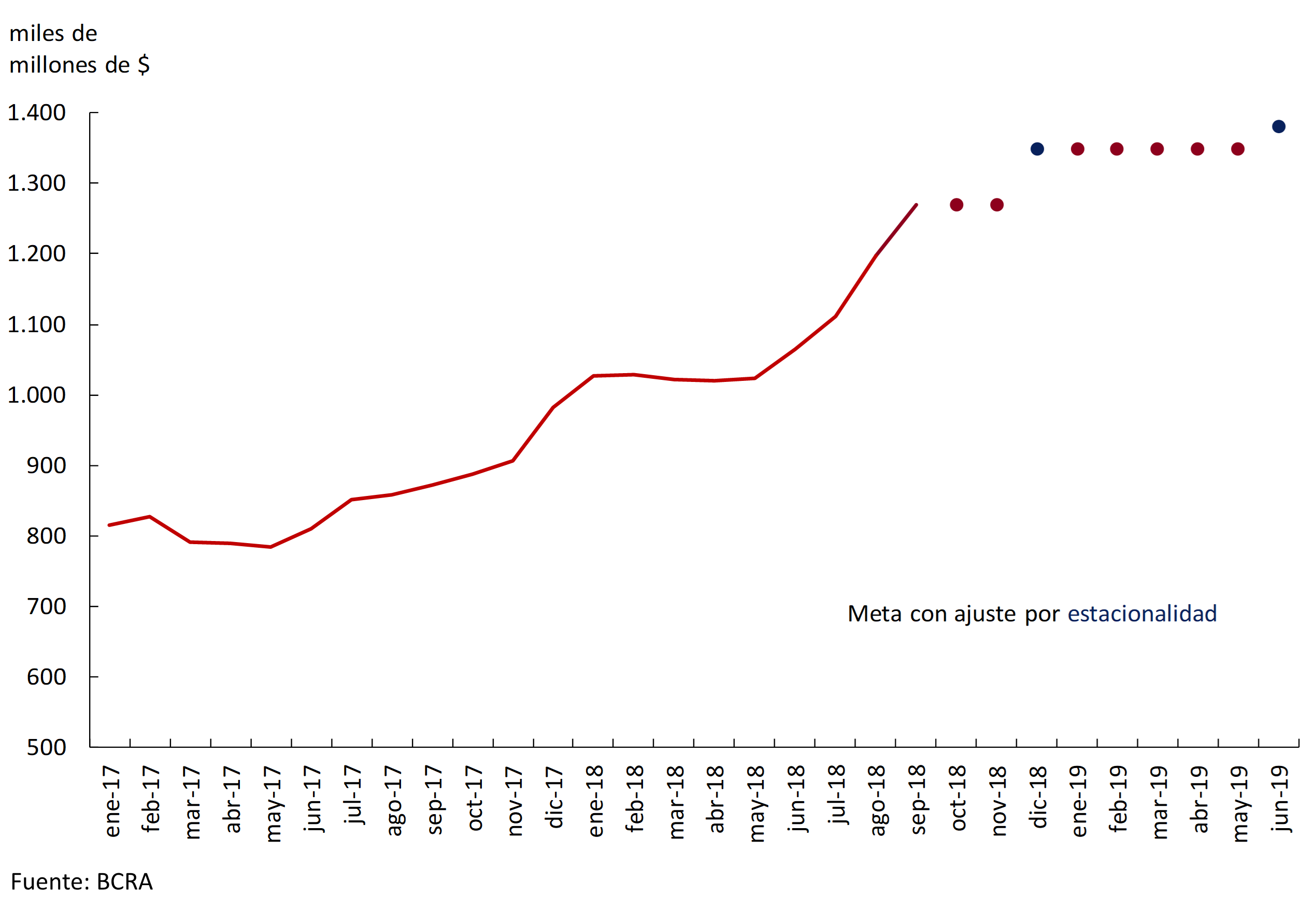
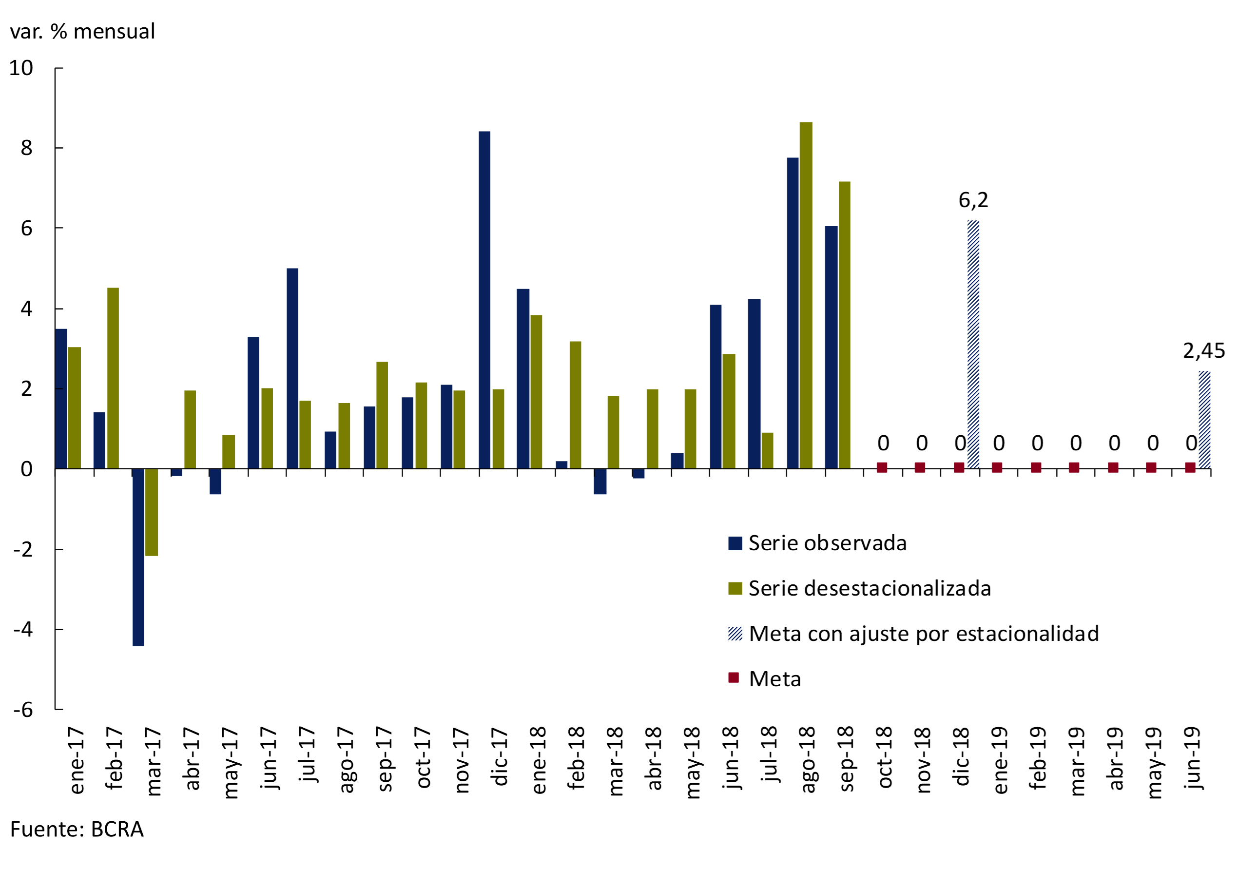
More specifically, the nominal anchor was established in the commitment not to increase the level of the monetary base until June 2019 (see Figures 5.4 and 5.5). The monetary base is composed of banknotes and coins issued by the Central Bank (held by the public and banks) and by the current account deposits of banks at the Central Bank (required by the minimum cash regulation). This monetary aggregate was chosen because it is the one that is under the direct control of the Central Bank. The goal of zero nominal monthly growth of the monetary base was defined on the monthly average of daily balances and will be adjusted with the seasonality of the months of December and June, when the demand for money increases, to avoid an excessive contractionary bias in monetary policy (a growth of the monetary base of 6.2% per month and 2.45% per month will be allowed in those months, respectively).
Figure 5.4 | Monetary base targets (October 2018 – June 2019). Average monthly balances
The aggregate target implemented implies a significant contraction in the growth of the quantity of money, since the monetary base has shown an expansion of more than 2% per month without seasonality in recent months, while it will now stop increasing (see Figure 5.5). Additionally, due to the recent dynamics of the exchange rate, the survey of market expectations predicts that inflation in the coming months will be high (although decreasing), so the monetary base will contract in real terms.
Figure 5.5 | Monthly nominal % change in the monetary base (observed until September 2018 and target between October 2018 and June 2019)
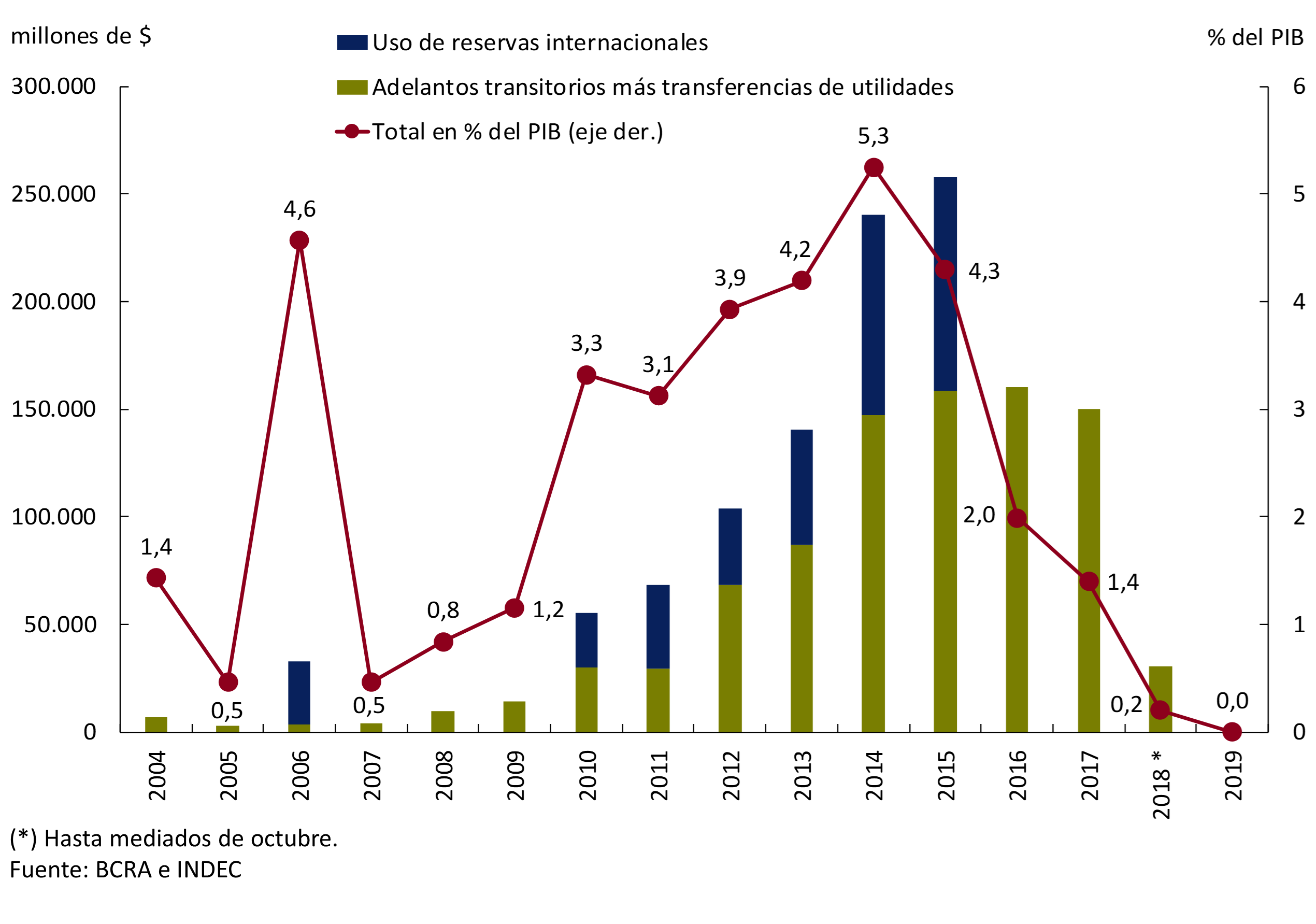
The new monetary policy is consistent with the primary fiscal balance in 2019 and surplus in 2020 targets set in the new agreement with the IMF. As announced in June of this year, the Central Bank will not make any more transfers to the Treasury. Up to that time, transfers had accumulated $69.9 billion, however, since then, transitory advances of $39.4 billion have been allowed to expire, bringing the amount transferred up to mid-October to 0.2% of GDP and will fall to zero in subsequent years (see Figure 5.6). The elimination of this source of monetary issuance reinforces the commitment to decreasing inflation over time.
Figure 5.6 | Transfers from the BCRA to the National Treasury
From an operational point of view, the monetary target is implemented through daily auctions of Liquidity Bills (LELIQ) with banks31. In this way, the reference interest rate came to be defined as the average rate resulting from daily operations. In turn, the monetary authority can inject or absorb liquidity through purchases or sales of LELIQ in the secondary market and limited its intervention in the pass market to operations with a 1-day term32.
By setting a target on the quantity of money, the interest rate of the LELIQ began to be determined by the supply and demand of liquidity, until it reached a level consistent with the commitment to zero growth of the monetary base. In any case, until there is evidence of a fall in inflation expectations 12 months ahead, the Central Bank will not let the interest rate of the LELIQ fall below 60% per year.
Likewise, if the reference rate becomes determined by the liquidity conditions of the money market, it could lead to greater variability of the reference rate. However, this is not expected to translate into higher volatility in the financial system’s deposit and lending rates due to several factors. First, we are starting from historically high levels of volatility in short-term interest rates (interbank calls, passes and 7-day advances). This is because when the Central Bank was setting the monetary policy rate, it was decided to expand the corridor of pass rates on several occasions starting in May and then the ceiling of said corridor was eliminated, which contributed to increasing the variability of market rates. Second, previous episodes of high volatility in shorter-term interest rates did not show significant increases in the volatility of interest rates on longer-term deposits or loans.
One difficulty facing the implementation of monetary policy in the previous months was the existing stock of LEBACs. The concern of economic agents regarding the risk of renewal, particularly of the holdings of the non-financial private sector, had become a factor of financial instability that was at the center of the scene during the exchange rate turbulence that began in April of this year. In this sense, the Central Bank will continue with the dismantling of LEBAC that began in August to completely eliminate its stock in December of this year. The monetary expansion generated by the reduction of LEBAC will continue to be absorbed by the Central Bank through reserve requirements and LELIQ to meet the growth target of the monetary base. Likewise, the Treasury will continue to contribute to this disarmament by issuing Bills, the proceeds of which will be mostly deposited in the Central Bank, through current account deposits with the monetary authority or the purchase of LELIQ by the Banco de la Nación Argentina.
5.2.2 Definition of intervention and non-intervention zones in the foreign exchange market as a complement to the monetary base target
Exchange rate flexibility allows countries to adapt to different external conditions or internal shocks (e.g., drought), which minimizes the cost to economic activity and employment. On the other hand, a negative shock that implies the need for an increase in the real exchange rate in a context of a fixed exchange rate leads to the difficult path of price deflation, as has been observed on numerous occasions in the past. However, recognizing the benefits of exchange rate flexibility does not imply ignoring the fact that excessive exchange rate volatility can be problematic, especially in our country, where the exchange rate plays a key role in the formation of inflation expectations, has a significant influence on the public’s portfolio decisions, and can generate episodes of strong uncertainty that negatively affect the level of activity in the economy. That is why the monetary target is complemented by the definition of areas of intervention and non-exchange intervention. The non-intervention zone was established for October 1 between $34 and $44, within which the peso floats freely, and is adjusted daily at a rate of 3% per month until the end of the year, a variation that will be recalibrated at the beginning of next year (see Figure 5.7).
Figure 5.7 | Scheme of non-intervention zones and foreign exchange intervention
In the event that the exchange rate is above the non-intervention zone (a sign of falling demand for financial assets in pesos), the Central Bank can hold daily foreign currency auctions for up to US$ 150 million. These sales result in a subtraction of pesos from the economy that tends to correct an excessive pressure towards the depreciation of the peso.
In the event that the exchange rate is below the non-intervention zone (a sign of increased demand for pesos), the Central Bank can buy foreign currency to avoid excessive appreciation of the peso. Faced with this sign of increased demand for money, the monetary authority may decide to increase the monetary base beyond the targets, supporting this expansion through an increase in international reserves.
It is important to emphasize that the boundaries between the intervention and non-intervention zones do not constitute fixed parities to which the Central Bank commits, but should be interpreted as guides on what can be expected from the behavior of the Central Bank in each zone. This scheme of intervention and non-intervention zones combines the benefits of floating exchange rates with the benefits of preventing excessive fluctuations in the exchange rate. The Monetary Policy Committee will review the slope and width of the non-intervention zone by the end of the year.
5.2.3 Consistency of the new monetary scheme
Below, a series of factors are described that show that the new monetary scheme is sustainable and that it gives a reasonable margin of maneuver to the Central Bank to meet its objectives.
Sustainability of the Central Bank’s remunerated liabilities in pesos
The new monetary scheme provides for the use of the LELIQ as a regulatory instrument for the liquidity of the economy. In this context, there are several factors that underpin the sustainability of these liabilities of the monetary authority. First, in recent months, the balance of bills, notes and passes of the Central Bank has been reduced both in terms of GDP and in terms of international reserves, which gives the starting point greater room for maneuver to the new monetary policy. Thus, between April and September, the weight of interest-bearing liabilities fell from 11.2% of GDP to 5.6% of GDP, while the ratio to international reserves went from 1.1 to 0.4 (see Figure 5.8). This dynamic was explained, first, by the fall in demand for LEBAC by the non-banking private sector since the beginning of the financial turbulence in April and, later, by the program to dismantle the stock of LEBAC implemented by the Central Bank as of August. In the case of the ratio to international reserves, the increase recorded by the exchange rate in that period also had an influence.
Figure 5.8 | BCRA bills, notes and passes in terms of GDP and international reserves
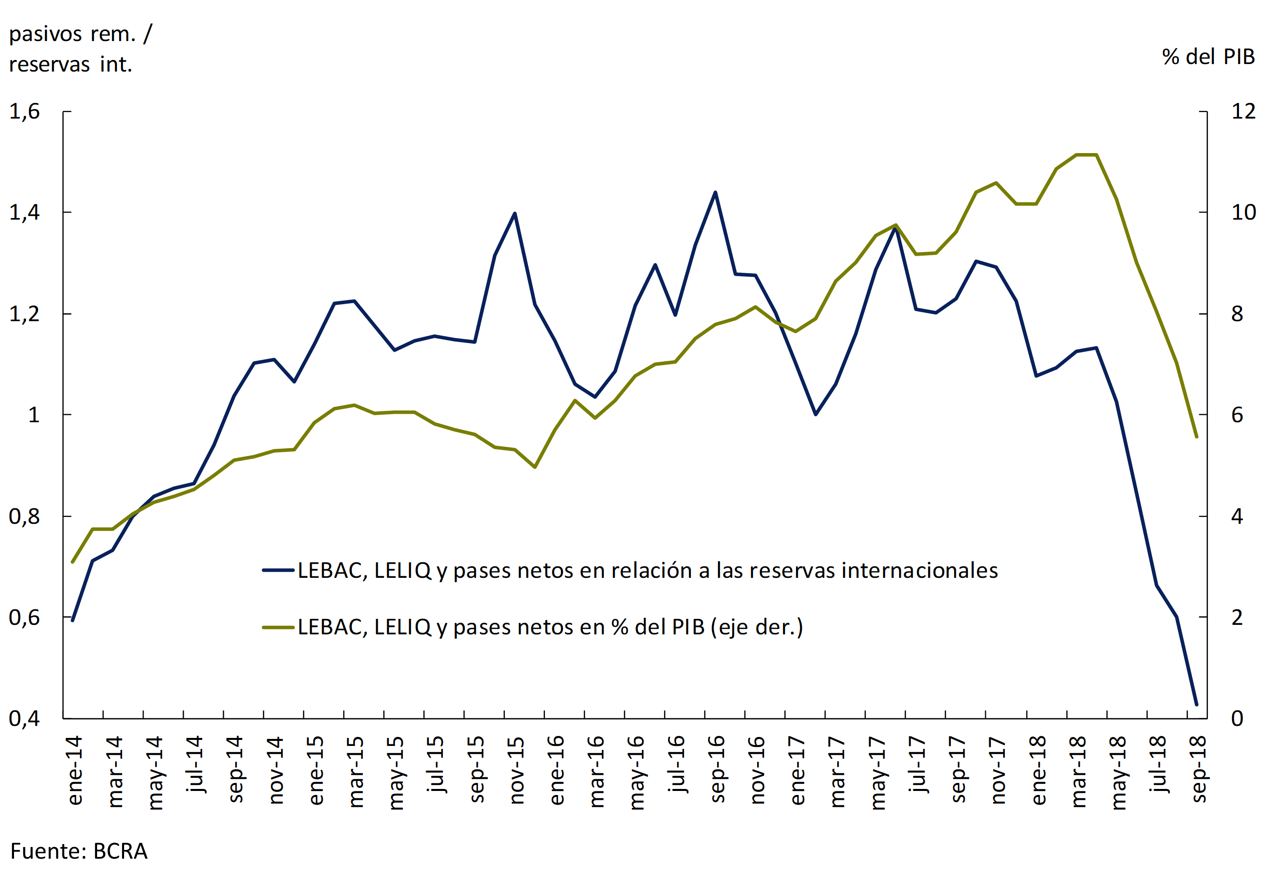
On the other hand, the factors of monetary base creation that in the past explained the increase in interest-bearing liabilities due to the need to sterilize a part of this expansion will not be present in this new stage. Thus, while net purchases of foreign currency (mainly from the public sector) and transfers to the Treasury for transitory advances and remittances of profits reached close to 4% of GDP between 2016 and 2017 (years in which the stock of LEBACs grew), neither foreign exchange purchases nor financing from the Treasury are expected for the coming years. in a context in which there is also a commitment by the National Government to stabilize the primary result in 2019 and achieve a surplus from 2020 (see Figure 5.9).
Figure 5.9 | Factors of expansion of the monetary base linked to operations with the National Treasury
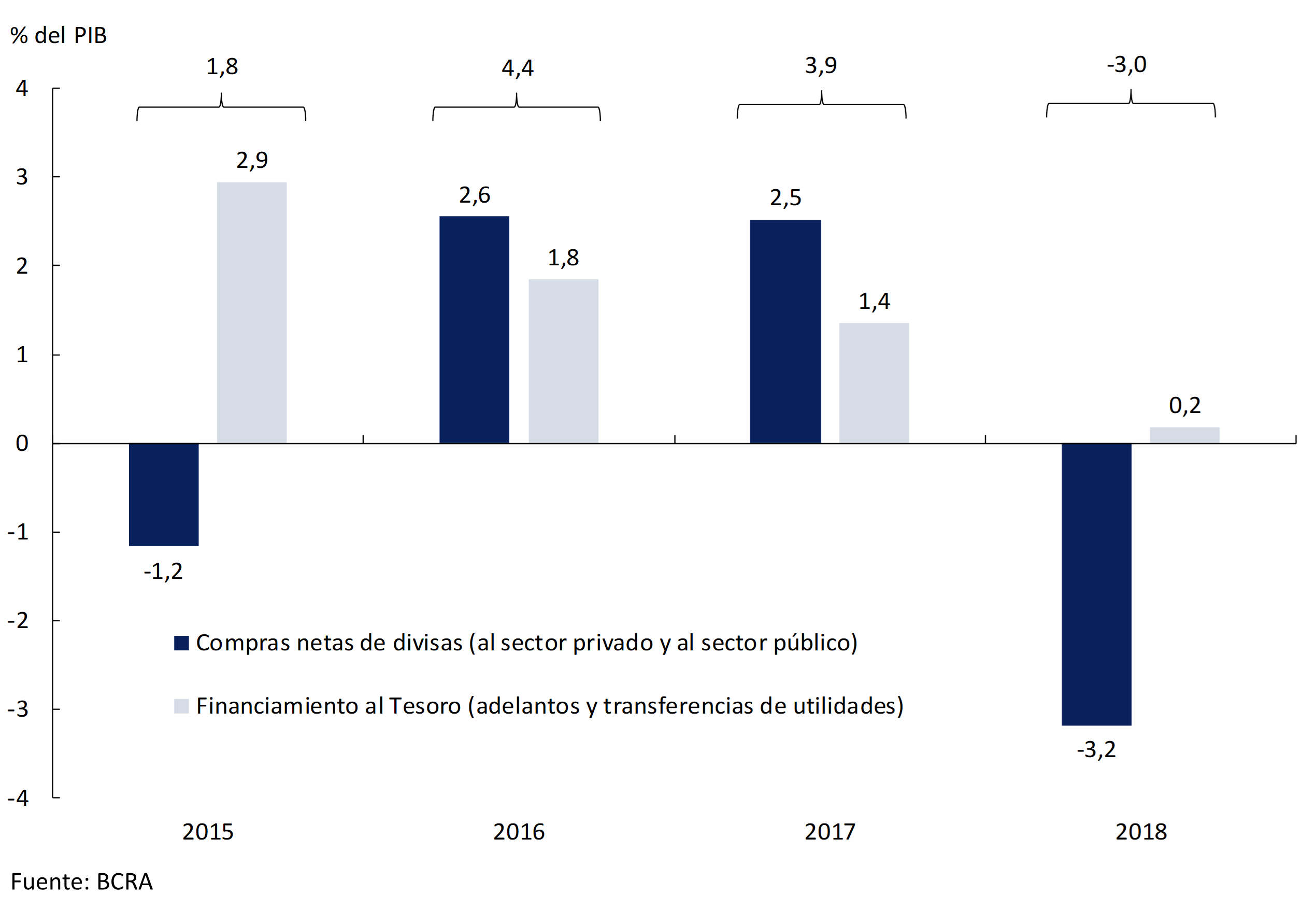
At the same time, LELIQs, unlike LEBACs, can only be acquired by banks, which gives greater stability to their demand compared to the rest of the economic agents due to the rules that financial institutions must comply with and dictated by the Central Bank itself.
Finally, meeting the monetary base target could require an increase in the interest rate of the LELIQs that would contribute to increasing their stock due to the need not to monetize interest payments in order to meet the monetary target. Even assuming an extreme scenario in which the real interest rate on LELIQs remains at current levels until the end of next year (real monthly effective rate of 1.5%), the ratio of remunerated liabilities to GDP would remain practically stable at around 6%. On the other hand, if an even more extreme scenario is considered, in which the nominal interest rate of the LELIQ remains at the current levels of 72% per year, the weight of interest-bearing liabilities in GDP would reach 7.8% in December 2019, which is still about 3.4 p.p. below the peak recorded in April of this year (see Figure 5.10).
Figure 5.10 | Evolution of the BCRA’s interest-bearing liabilities in terms of GDP with scenarios of constant nominal and real interest rates
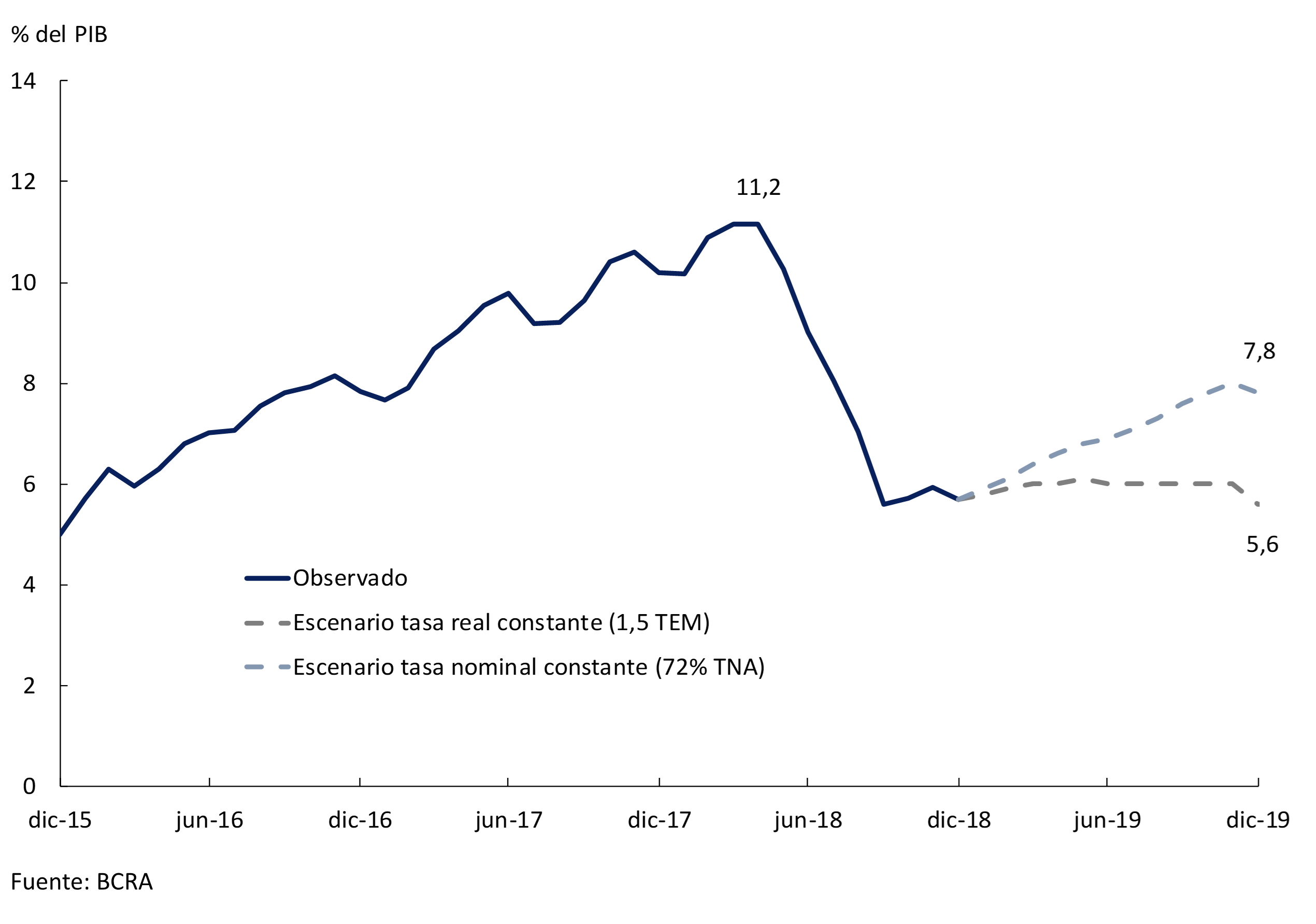
Sustainability of the exchange rate scheme: real exchange rate level and daily currency auctions
With regard to the exchange rate scheme, a number of factors contribute to the consistency of the exchange rate values chosen to define the intervention and non-intervention zones and of the daily auction scheme in the event that the exchange rate exceeds the upper limit of the non-intervention zone.
After the increase in the nominal exchange rate recorded in the year, the real exchange rate is at levels more consistent with macroeconomic balance. In this context, the multilateral real exchange rate at the upper limit of the non-intervention zone is at 2003 levels, when the exchange rate had overreacted to the collapse of convertibility. Likewise, the terms of trade are currently 35% higher than those recorded at that time, which would imply the need for a lower real exchange rate than in 2003 to balance the external accounts. On the other hand, the multilateral real exchange rate corresponding to the lower limit of the non-intervention zone is at similar levels in mid-2011, when the economy registered a substantially lower current account balance imbalance than it is today and with terms of trade at levels similar to those of today (see Figure 5.11).
Figure 5.11 | Multilateral real exchange rate, terms of trade and limits of foreign exchange non-intervention zones33
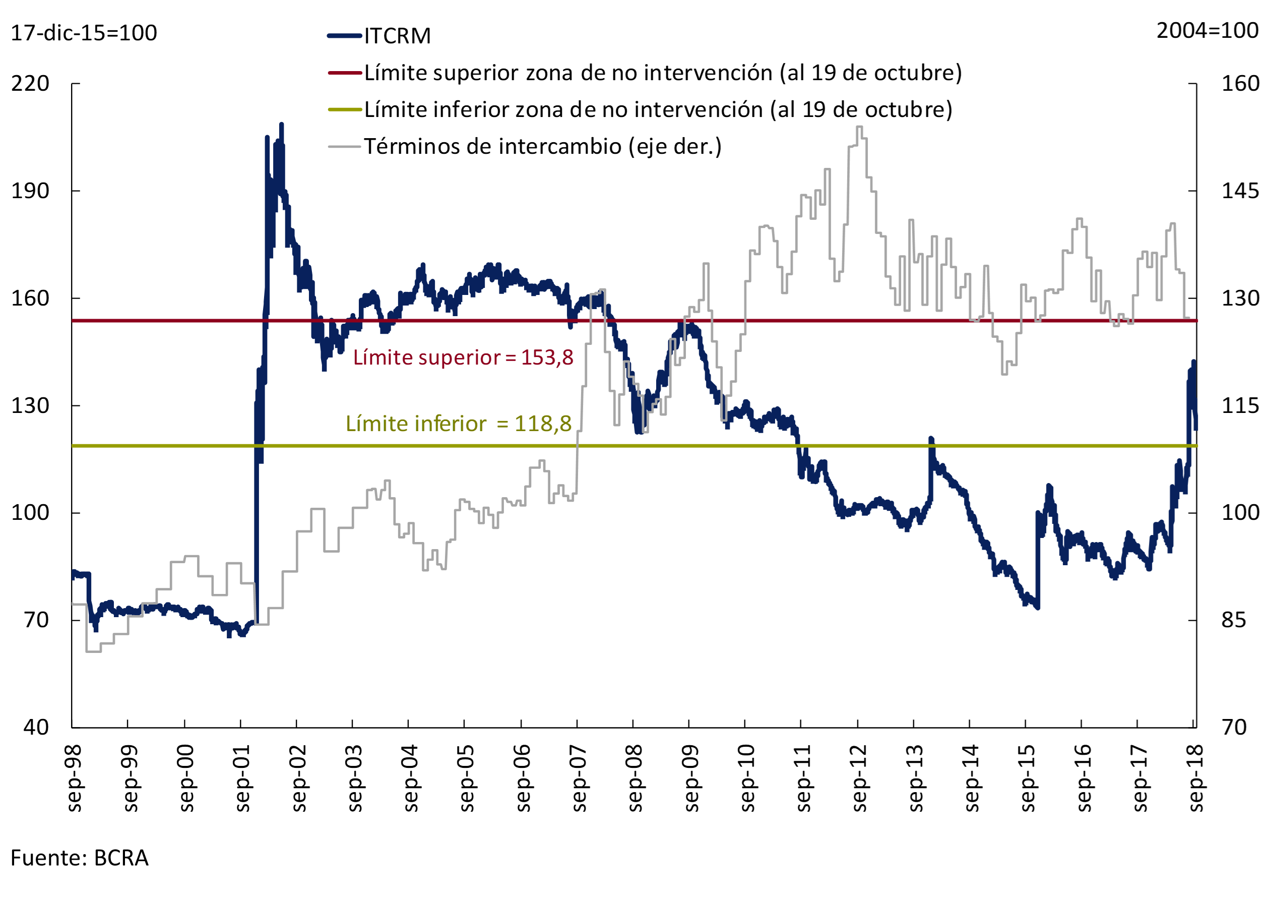
On the other hand, the current level of the real exchange rate is contributing to the adjustment of the external accounts, in addition to the effect of lower economic activity on import demand (see Section 3). In fact, in recent weeks there has been a lower daily demand for foreign currency from net importers, for hoarding and tourism, which are very relevant items in the explanation of the outflow of foreign currency from the economy (see Figure 5.12)34. Likewise, not only is the supply of dollars expected to react positively to the new level of the real exchange rate, but also that next year’s exports of cereals and oilseeds will leave behind the impact of the drought. To this is added an income of dollars agreed with international organizations, as a result of the recent agreement signed with the IMF. Thus, during the rest of 2018 the Treasury will receive approximately US$ 13,440 million in disbursements from the IMF’s Stand-By Loan and US$ 1,513 million from other organizations, while in 2019 it will receive approximately US$ 22,820 million in disbursements from the IMF’s Stand-By Loan and around US$ 3,000 million from other multilateral organizations.
Figure 5.12 | Daily foreign exchange demand from net importers, hoarding and tourism (20-day moving average) and exchange rate
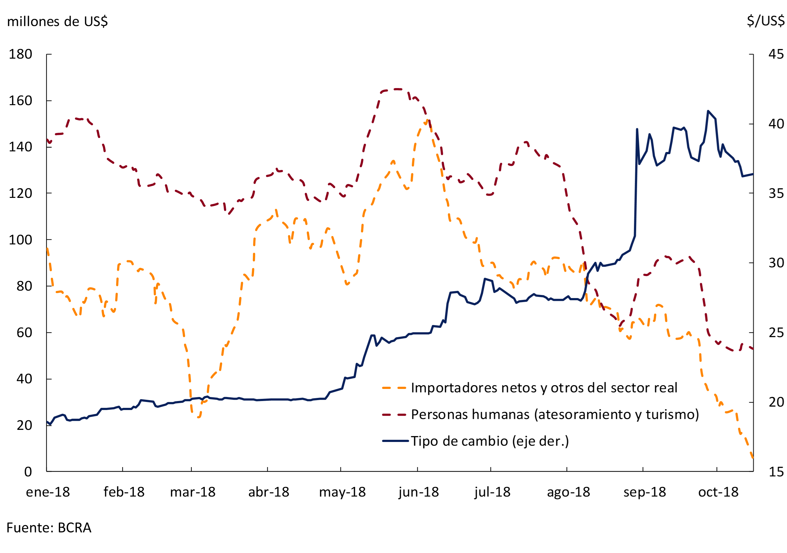
In the case of the Central Bank’s daily foreign exchange auction mechanism, defined for the upper limit of the non-intervention zone, the closest precedent is the daily auctions of the National Treasury implemented during July and the first days of August. These auctions, which in general were for amounts of less than US$ 150 million, were successful in stabilizing the foreign exchange market in a context of a less competitive exchange rate and with levels of demand for foreign currency much higher than the current ones (see Figures 5.1 and 5.12). These auctions were not accompanied by interventions by the Central Bank which, unlike those of the Treasury, have the potential to reduce the monetary base, which additionally contributes to stabilizing the foreign exchange market.
Limited impact of the new monetary scheme on the financial system
The financial system has shown great solidity throughout the episode of exchange rate turbulence that began in April, mainly reflected in the good performance of deposits in domestic and foreign currency during the period (see Section 5.3.3). In this context, there are several current characteristics of the financial system that lead us to think that there is room for maneuver in monetary and exchange rate policy so that they can meet their objectives without affecting banks in a relevant way.
First, while some increase in non-performing loan ratios in the financial system is expected as a result of current interest rate levels and lower levels of economic activity, non-performing loans are at low levels both historically and internationally, while banks are experiencing high levels of forecasting that exceed the amount of distressed loans (see Figure 5.13).
Figure 5.13 | Irregularity Ratio (IR) of Private Sector Credit (*) and Forecasting (**) – Financial System
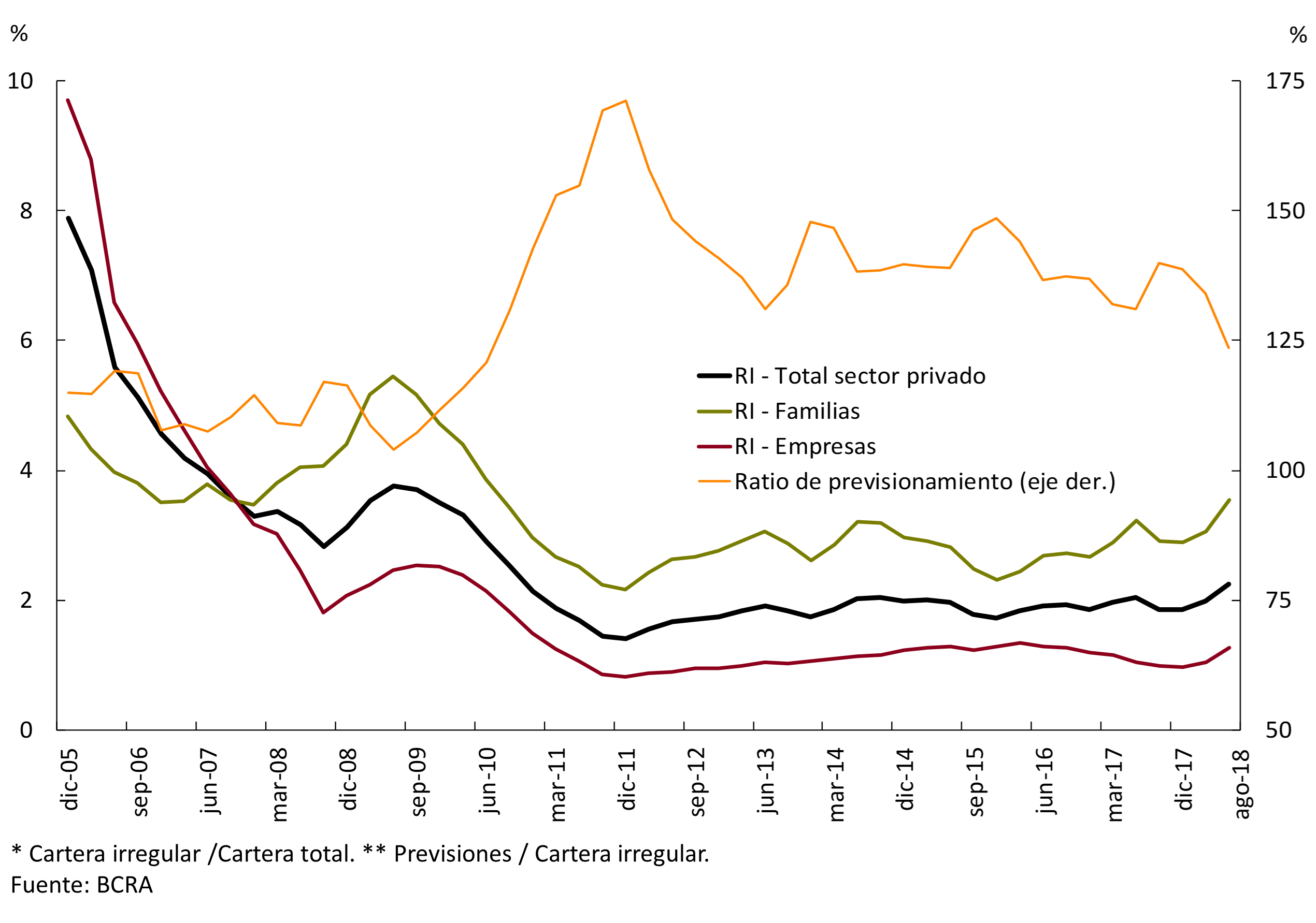
On the other hand, the rise in domestic interest rates and the increase in minimum cash ratios derived from the policy actions necessary to meet the new monetary base targets occur in a context in which the profitability of the financial system is maintained. The financial system is also showing high solvency indicators, with all financial institutions registering excess capital in relation to the minimum required by prudential regulation (see Figure 5.14).
Figure 5.14 | Solvency of the financial system (integration of regulatory capital in terms of risk-weighted assets)
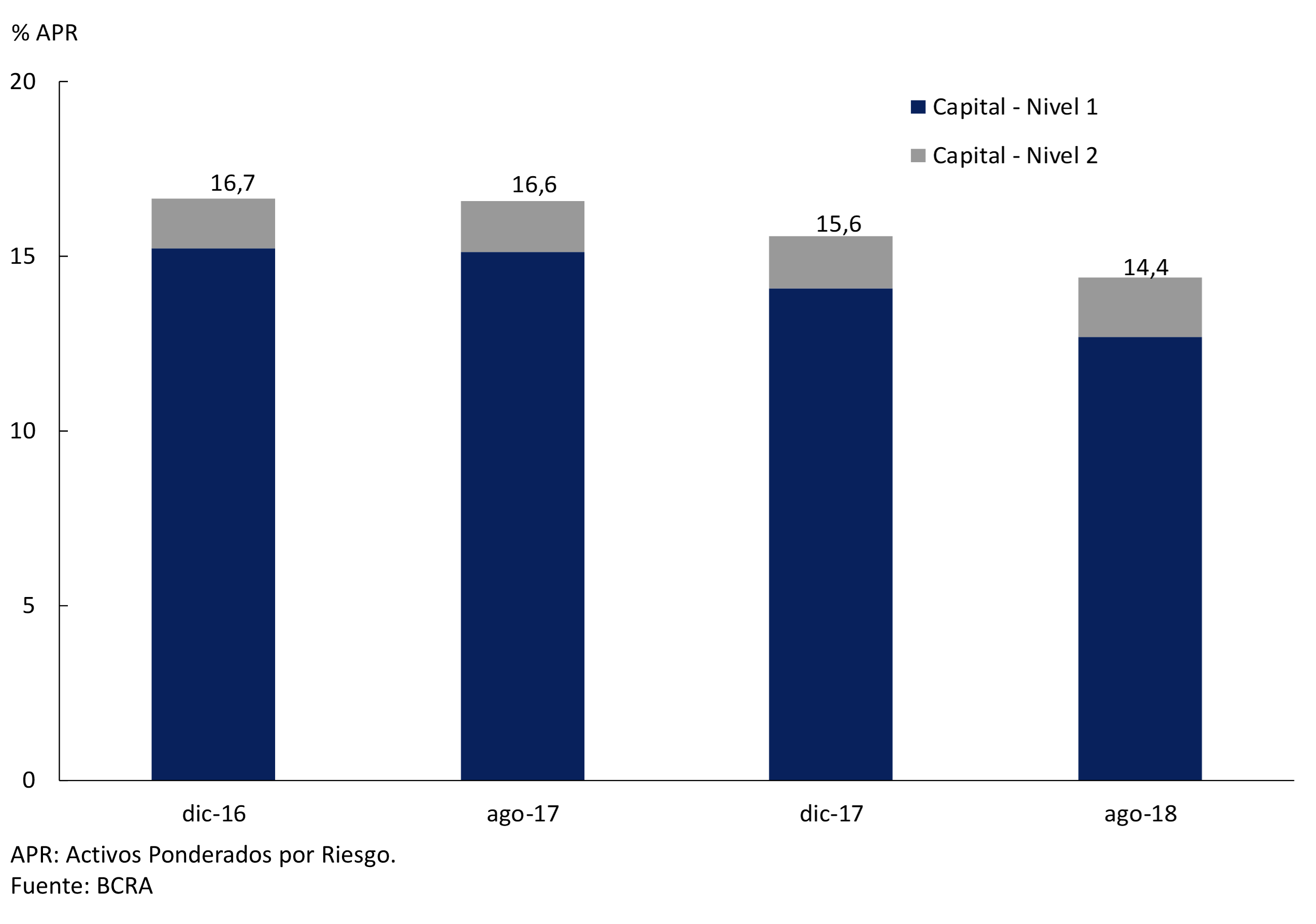
Finally, the low mismatch of foreign currency and the low levels of dollarization of the balance sheet of the financial system are consistent with the exchange rate flexibility implicit in the new scheme of intervention and non-intervention zones, so that potential movements in the exchange rate would not have disruptive impacts on the soundness of the banks. Thus, the currency mismatch, measured as foreign currency assets minus foreign currency liabilities plus net forward purchases of foreign currency, reached a level of 14.9% of eligible equity liability and 0.9% of bank assets in August (see Figure 5.15).
Figure 5.15 | Mismatch of currencies in the financial system (EM Asset – EM Liability + Net forward purchases of EM without delivery of underlying)
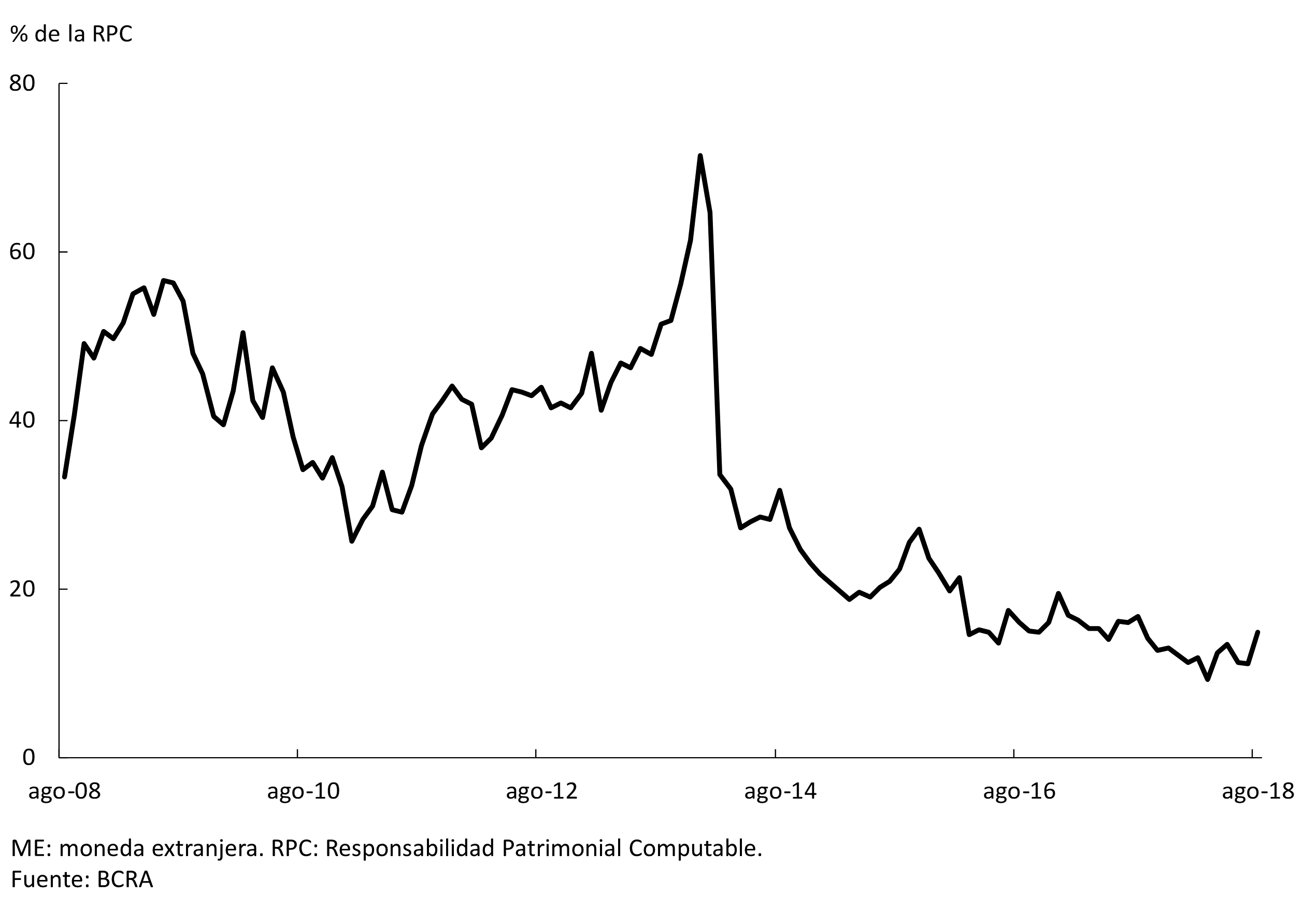
Limited impact of potential interest rate increases on the financing needs of the National Treasury
With regard to the possible impact of a restrictive monetary policy on the sustainability of the public accounts, the peso debt of the National Public Sector, which is subject to domestic interest rate risk, showed at the end of March of this year a low participation in the total debt held by private creditors of around 18% (latest available data). of which 5% correspond to variable-rate debt and 13% to fixed-rate debt (includes adjustable and non-adjustable debt by CER). In this sense, an increase in the interest rate in pesos of 10 p.p. would generate a growth in interest payments of only 0.07% of GDP in the case of variable-rate debt and 0.17% of GDP on the maturity of short-term debt in national currency on a net payment of interest on debt of 3.2% of GDP projected for 2019 according to data from the National Budget.
5.2.4 First results of the new monetary regime
The implementation of the new monetary regime as of early October restored calm to the foreign exchange market. The exchange rate moved downward within the hands-off zone, registering an 11% drop between September 28 and October 19 (see Figure 5.7). Thus, the exchange rate has risen by 95% since the end of last year, which places the real (multilateral) exchange rate at mid-2010 levels (see Figure 5.11).
With regard to the money market, prior to the start of the new monetary scheme, the Central Bank defined an increase in the interest rate of the LELIQ from 60% to 65% per year on September 28. As a complement to the above and in anticipation of the disarmament of LEBAC in mid-October, a series of measures related to minimum cash requirements were announced. On the one hand, it was decided to increase reserve requirements by 3 p.p. for the largest institutions in the system to be integrated with NOBAC or LELIQ, and that the entire minimum cash requirement on the increase in fixed-term deposits can be integrated with NOBAC or LELIQ, in order to encourage an increase in passive interest rates and to stimulate the capture of new fixed-term deposits by the entities35.
Finally, on October 1, the LELIQ daily bidding mechanism began to be implemented, which the Central Bank uses as the main instrument for meeting the aggregate target. With this new scheme, the LELIQ interest rate increased to a maximum of 73.52% on October 8 and then fell to 72.5% annually by the end of the third week of the month, which translates into a real interest rate (ex ante) that is at the highest levels in recent years (see Figures 5.2 and 5.16). As a result of the auctions held, the stock of LELIQ remained practically stable at around $ 450,000 million until the day before the third operation of LEBAC dismantling in mid-October (see Figure 5.16).
Figure 5.16 | Reference interest rate and stock of interest-bearing liabilities held by financial institutions (net passes, LEBAC and LELIQ)
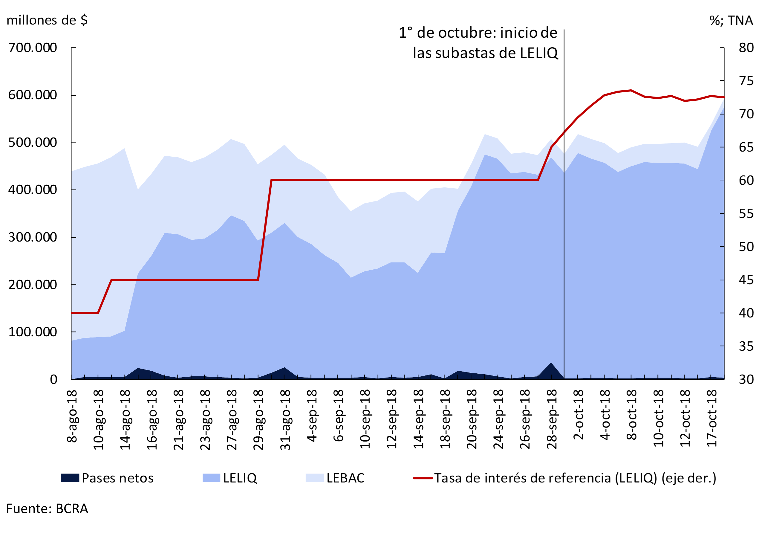
In this context, the monetary authority has been meeting the monetary base target for the month of October. Although the goal is defined for the monthly average of daily balances, a preliminary assessment of its compliance can be made for the first three weeks of the month. Thus, the average of the daily balances until the 21st ($ 1,256 billion) is $ 15,000 million below the average of daily balances recorded in September ($ 1,271 billion). Because the monetary base has a marked intra-month seasonal behavior (with a higher level at the beginning of the month than at the end of it), it is useful for monitoring the goal to compare the evolution of the monetary base with that of the same period of the previous month. Thus, the cumulative average of the monetary base during the first three weeks of October was $24,500 million lower than in the same period of September (see Figure 5.17). This reduction required an additional effort in this period, since in the first two weeks of September the coefficient of unpaid reserve requirements was lower. If the monetary base for September were corrected for this factor, the average for October to the 21st would be $ 60,500 million lower than that of the same period in September.
Figure 5.17 | Compliance with the monetary base target as of October 21
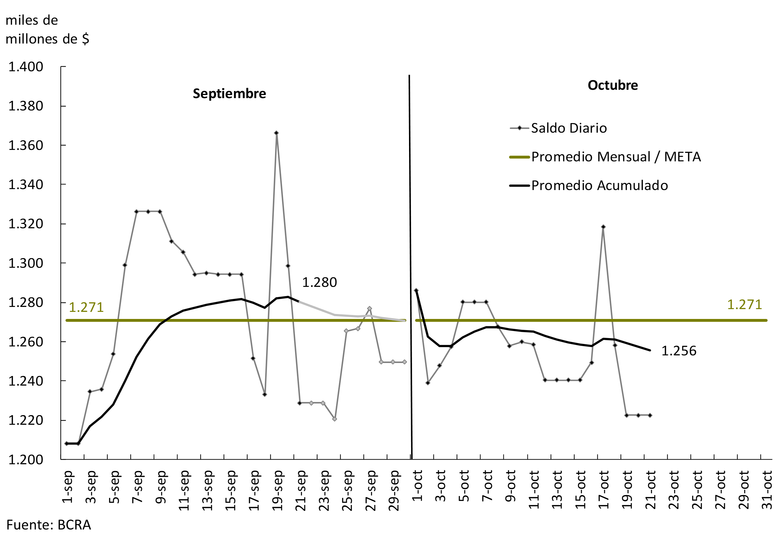
For their part, international reserves reached US$ 48,300 million in mid-October, a level similar to that of the average for 2017 and similar to the floor observed on June 21, prior to the first disbursement by the IMF of US$ 15,000 million (see Figure 5.18).
Figure 5.18 | BCRA International Reserves
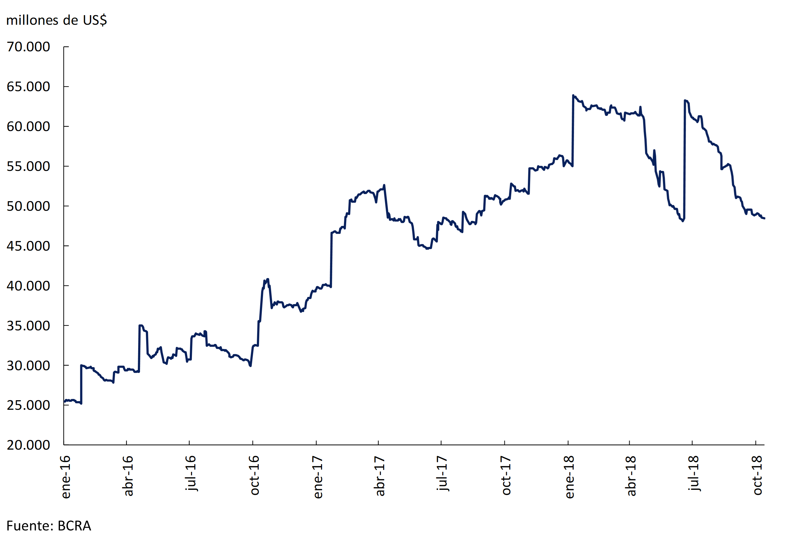
Although inflation expectations, as measured in the Central Bank’s Market Expectations Survey, have grown since the beginning of the exchange rate turbulence and are at high levels, it is noteworthy that the market continues to expect a slowdown in inflation at 12 and 18 months, also considering that the last survey corresponding to September was after the announcement of the new monetary scheme (see Section 4). In this context, it is expected that the monetary contraction generated by the new monetary policy scheme, together with the confirmation of the downward path of the primary result and the commitment assumed not to finance the Treasury anymore, will begin to be reflected in a fall in inflation expectations and inflation rates in the coming months.
5.3 Impact of exchange rate turbulence and Central Bank measures on the financial system
5.3.1 Money Market Interest Rates
Interbank market interest rates accompanied the increases in the reference rate, registering high volatility during the exchange rate turbulence in July and August, which moderated from September after the decision on August 30 to increase the LELIQ rate to 60% annually (see Figure 5.19). During the first days of October, the month that began the implementation of the new monetary policy scheme, the LELIQ rate reached an average of 71.9% per year, increasing by about 12 p.p. compared to the average for the month of September. This increase was partially transferred to the 1-day call and third-party pass rates, which exhibited an average increase of around 9 p.p. and 7 p.p., respectively, during this period, and accumulated an increase of 30 p.p. and 25 p.p. compared to June, respectively.
Figure 5.19 | Money Market Interest Rates
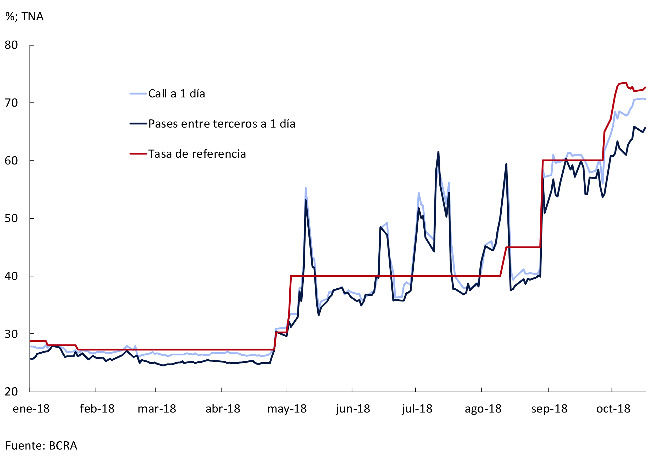
5.3.2 Deposit and Loan Interest Rates
In line with the tightening of monetary policy ordered by the Central Bank, interest rates on private sector time deposits in financial institutions showed an upward trend in the third quarter, a rise that accelerated in the first days of October. It should be noted that the policy of allowing financial institutions to integrate part of the reserve requirements with LELIQ or NOBAC, mainly for time deposits, encouraged a greater capture of this type of deposits, which was reflected in the system’s passive interest rates. As a result, between June and the first days of October, the TM20 and BADLAR offered by private banks increased by 21 p.p. and 19 p.p., reaching average levels of 53.2% per year and 49.6% per year, respectively, while the rate on retail fixed terms increased by 16 p.p. to 42.2% per year (see Figure 5.20)36. Regarding the interest rate for fixed-term deposits adjustable by UVA, the average rate stood at 4.7% annually in September, increasing 0.5 p.p. during the quarter.
Figure 5.20 | Main Passive Interest Rates of Banks
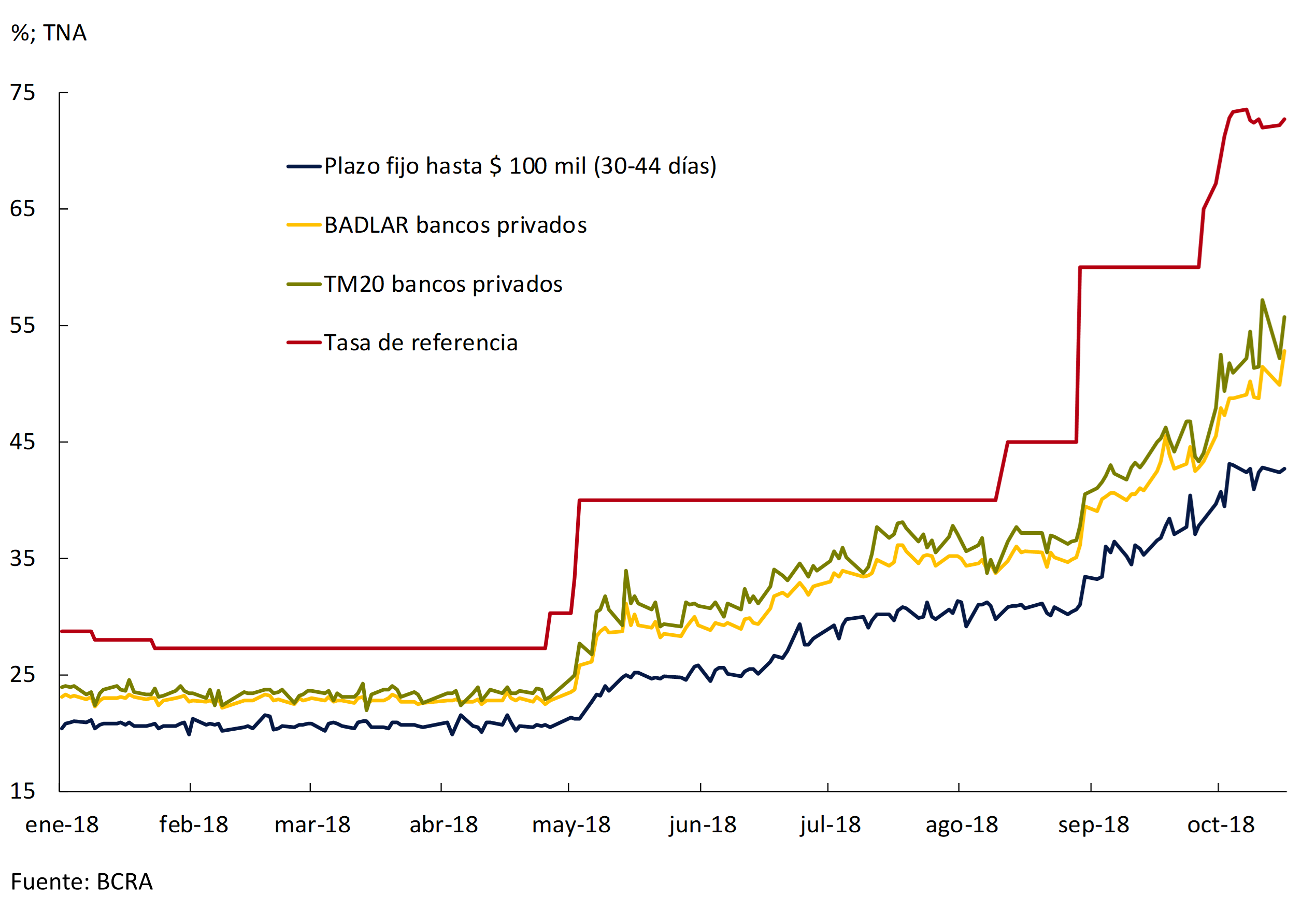
The rates of the main financing lines of financial institutions remained in line with the increases in the remaining money market rates, with increases in short-term loans to companies standing out (see Figure 5.21). Thus, interest rates on advances and discounted and signature documents increased on average between June and the first days of October by 34 p.p., 24 p.p. and 24 p.p., reaching average levels of 77%, 62% and 61% per year, respectively. On the other hand, personal and pledge loans rose by 18 p.p. and 9 p.p. in that same period, taking average values of 62% and 30% annually in the first days of October. In relation to UVA-adjustable loans, during the third quarter the mortgage rate remained at around 6% per year, while personal and pledge loans increased by 1.6 p.p. and 1.4 p.p. in the period, reaching average rates of 14.5% and 14.7% per year, respectively.
Figure 5.21 | Main lending rates of banks

5.3.3 Bank deposits, loans and liquidity
The financial system has shown clear signs of solidity in recent months. This was reflected, firstly, in the behavior of private sector deposits in pesos, which increased nominally by 3% per month without seasonality during the third quarter of the year, a higher rate than that recorded in the first half of the year (see Figure 5.22). This increase was observed in both demand and fixed-term deposits, although the latter, which better reflect savings decisions, exhibited greater dynamism, with an average nominal growth of 3.3% per month compared to 2.6% per month for the former. This increase in term deposits in the third quarter can be attributed to the rise in passive interest rates and the LEBAC cancellation program. During the first 9 months of the year, fixed-term deposits in pesos in the private sector grew by 24.9% against 19.5% of demand deposits (values without seasonality). For its part, public sector deposits in pesos also showed a strong upward trend during this third quarter of the year, driven by the dollar auctions carried out by the Treasury and by the LEBAC disarmament funds raised with Treasury Bills, growing at a rate of 7.1% per month in nominal values and accumulating in these first 9 months of the year a rise of 109%. Thus, total deposits in pesos nominally increased by an average of 4.2% per month during the third quarter of the year (without seasonality).
Figure 5.22 | Private sector deposits in pesos (average monthly variation in the quarter – nominal without seasonality)

Private sector dollar deposits also showed an upward trajectory during the quarter, increasing on average by 1.3% in original currency. Although towards the end of August and the beginning of September, in line with the moments of greatest exchange rate tension of the quarter, a fall in these deposits was observed, from mid-September this dynamic began to reverse, continuing in this way during the first days of October (see Figure 5.23). Thus, the stock of foreign currency deposits of the private sector averaged about US$ 27,200 million in the first days of October, about US$ 1,500 million above the level at the end of 2017.
Figure 5.23 | Private sector deposits in foreign currency
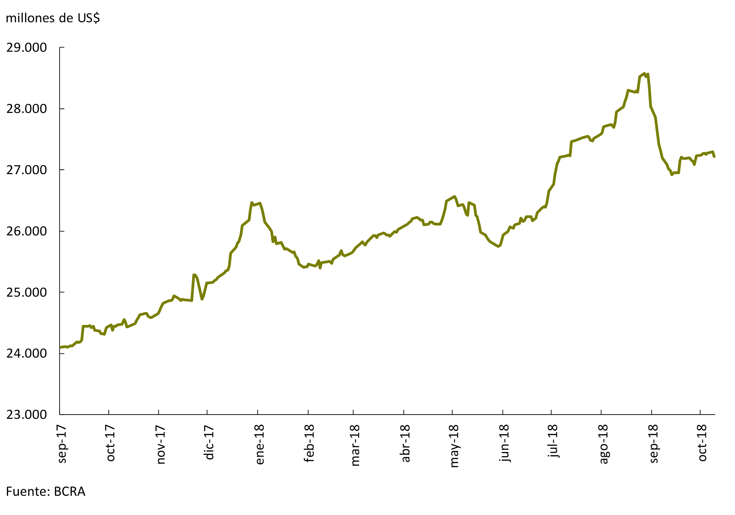
In the third quarter, credit from the financial system to the private sector exhibited less dynamism compared to previous quarters. In the peso segment, average monthly nominal growth in the third quarter fell to 1%, while in real terms it showed an average monthly contraction of 2.5% without seasonality (see Figure 5.24). Thus, the nominal year-on-year growth rate fell from 50% in June to 39% in September. The contraction compared to the previous quarter was observed in a generalized way in all credit lines, with documents, pledges and personal leading the retraction. On the other hand, financing in dollars also reversed the growing trend they had been showing in previous quarters and fell by an average of 0.5% per month in source currency during the quarter (compared to an average expansion of 1.8% per month in the first half of the year).
Figure 5.24 | Loans to the private sector in pesos (average monthly variation in the quarter – real without seasonality)
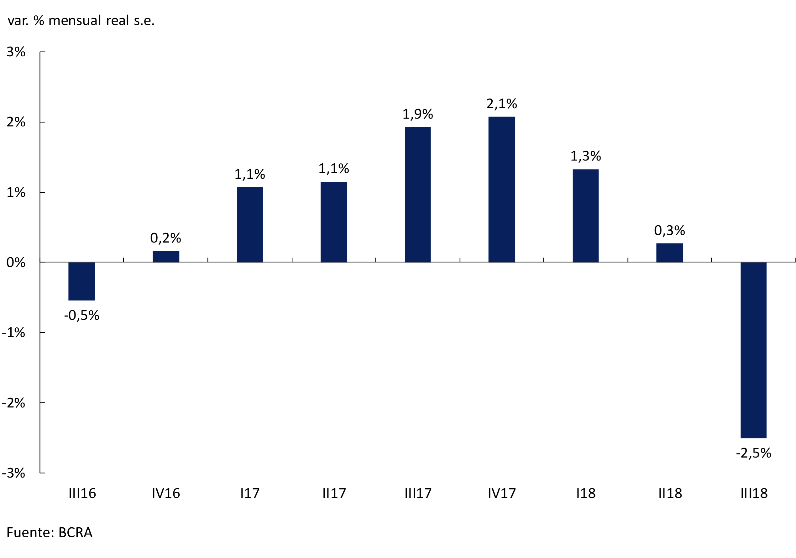
The increase in deposits and the lower dynamism of loans, together with the increase in reserve requirements ordered by the Central Bank, continued to increase the ample liquidity in pesos of financial institutions during the quarter (+3.7 p.p.), which reached 47.1% in terms of deposits in September (see Figure 5.25)37. Likewise, within the framework of the LEBAC cancellation program and the entry into force of increases in minimum cash requirements (part of which can be integrated with Central Bank securities), an increase of 12.7 p.p. was observed in the quarter in LELIQ’s holdings, both those affected by the integration of reserve requirements (+8.2 p.p.) and those of free availability (+4.6 p.p.). and current accounts at the Central Bank (+6 p.p.) to the detriment of LEBACs (-16.1 p.p.). Finally, by virtue of the aforementioned increases in reserve requirements, the surplus or voluntary liquidity of the institutions (net passes, LEBAC and non-integrable LELIQ) decreased by 12.3 p.p. in the quarter, reaching 9.5% of deposits in September.
Figure 5.25 | Liquidity of financial institutions
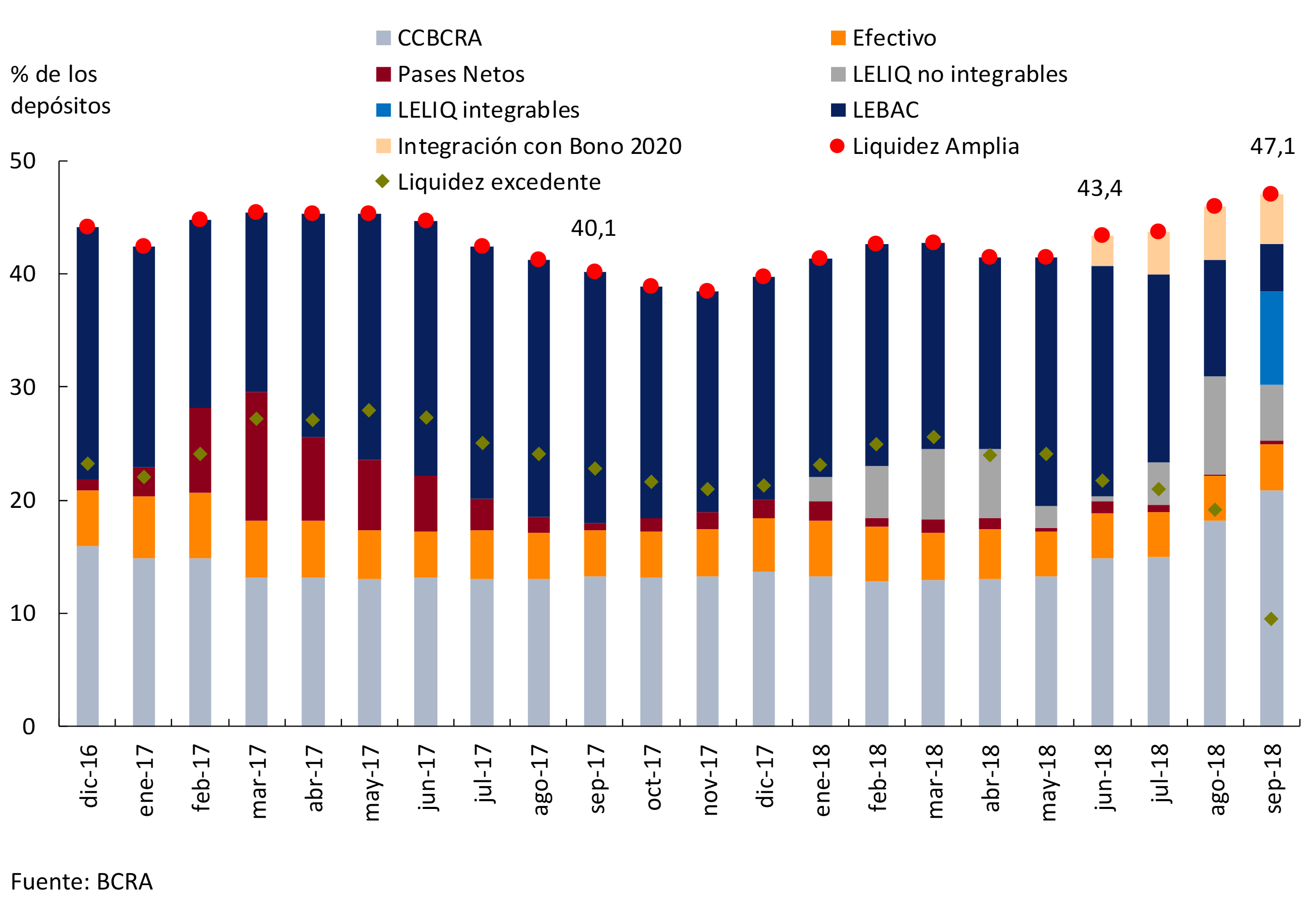
Section 1 / Developments in the energy sector
Argentina’s energy matrix is heavily dependent on gas. The production of refined gas – which accounts for about half of secondary energy production – is not enough to supply a growing demand, with a quarter of the gas consumed annually being imported.
Almost two-thirds of these imports come from Bolivia’s state-owned company, 38 but when consumption peaks in winter, it is necessary to resort to more expensive sources, such as purchases of liquefied natural gas (LNG). LNG vessels from Qatar, Trinidad and Tobago, Nigeria or Australia arrive at the regasification plants operating in the ports of Escobar and Bahía Blanca and dump more gas into the grid. 39 In addition, due to the lack of gas between April and September, electricity generating plants use liquid fuels (more expensive and less efficient) such as diesel and fuel oil, which are purchased abroad. These plants are the main demanders of natural gas in the system, followed by residential and industrial consumption (see Graph 1).
Graph 1 | Energy balance simplified. In tonnes of oil equivalent
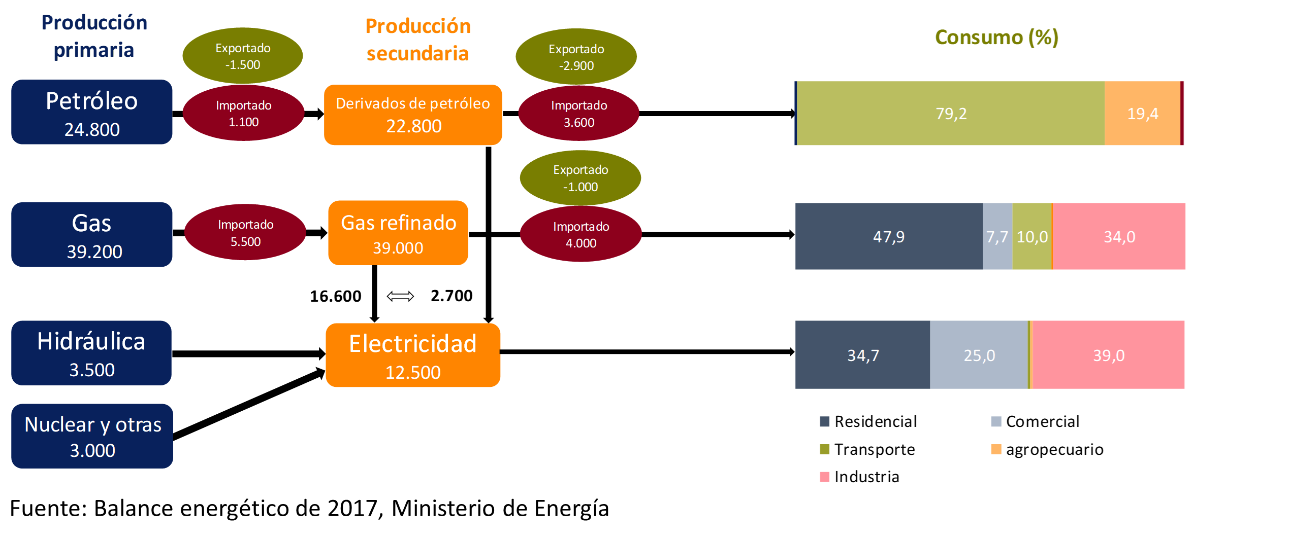
The energy policy adopted between 2003-2015 played a central role in the erosion of surplus results in the external and fiscal accounts (Navajas, 2015:40). Generalized energy subsidies showed a growing share of government spending, and distortions in relative prices led to an incentive to demand and a discouragement to supply, resulting in an increase in energy imports to cover the consumption gap.
In the gas sector, the downward trend in local production from 2008 onwards led to a constant deterioration in the sector’s trade balance, reaching a deficit equivalent to 1.1% of GDP in 2014 (see Graph 4). This in turn had an impact on the public accounts, due to higher energy imports by public companies and growing subsidies to demand41.
This declining trajectory of gas production began to be gradually reversed from 2014, with the application of various stimulus plans granted to investment. 42 Thus, from the minimum levels observed in 2014 to July 2018, total gas production accumulated an increase of 19.5%. This strong dynamism was explained by the extraction of unconventional gas43, placing total production at levels similar to those of 2009, still below historical maximums (see Graph 2).
Graph 2 | Primary production of natural gas
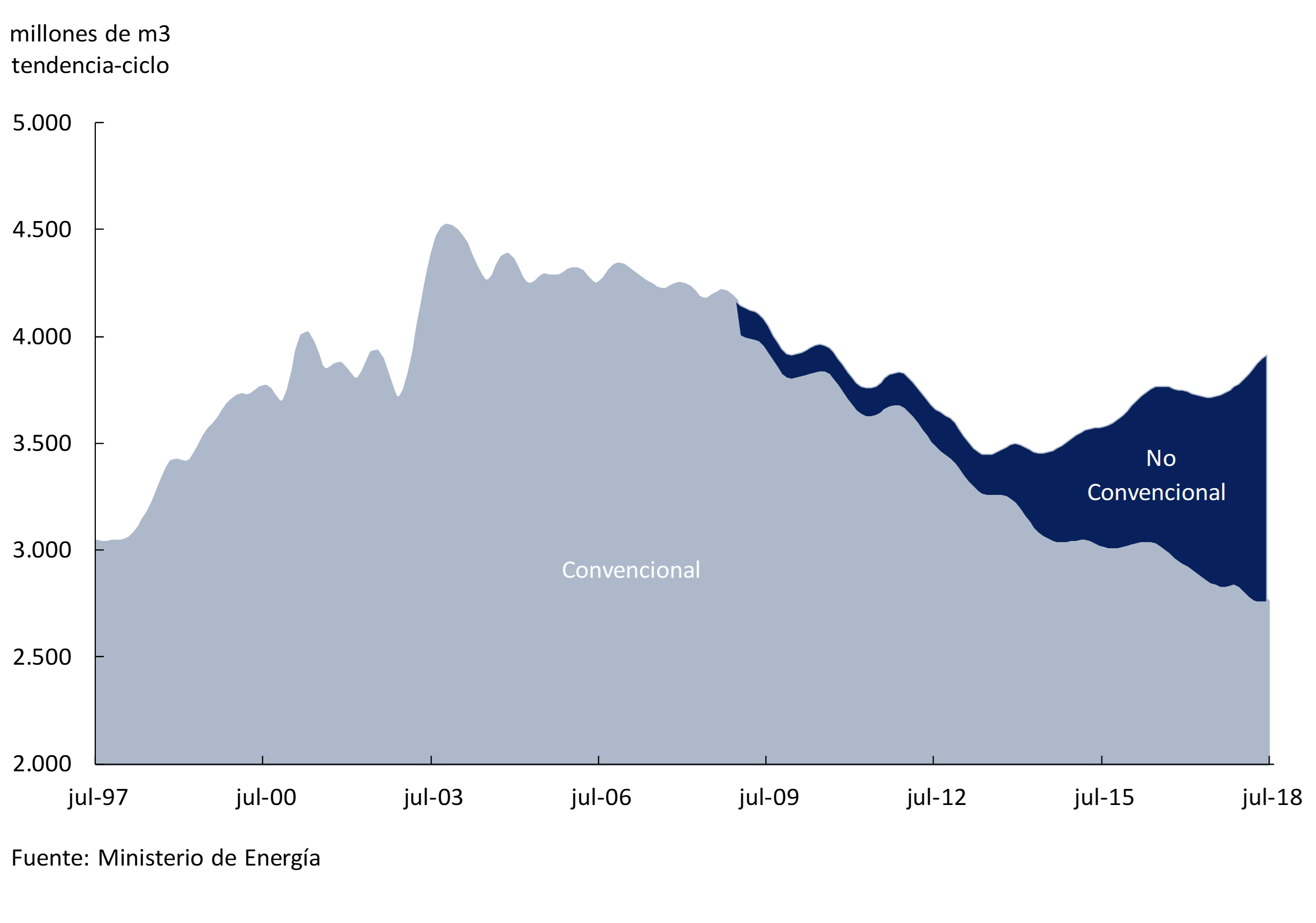
Between 2015-2017, the recovery of local gas production made it possible to replace 8% of the quantities imported44 and considerably reduce external purchases of liquid fuels for electricity generation concentrated in the winter months. According to CAMMESA data, the availability of gas in thermal power plants in the June-July two-month period increased by 32.2% YoY in 2017 and by 5.1% YoY in 2018, reducing imports of diesel (mostly imported) by 50% in the last two years (see Graph 3).
Graph 3 | Fuel consumption for electricity generation
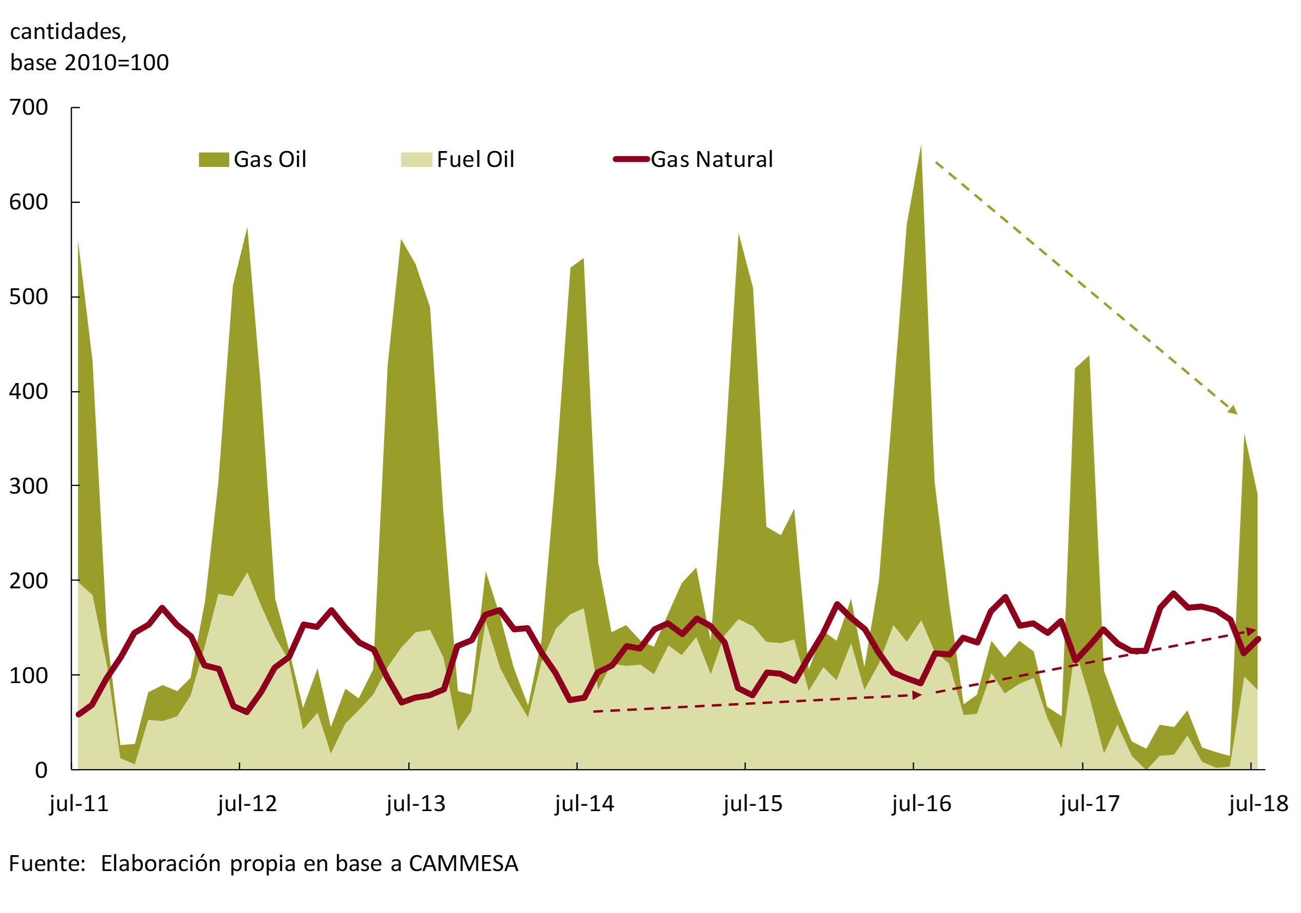
In order to expand gas production and replace LNG imports during the peak of local consumption in the winter period and given their limited storage capacity, producers need to increase external demand in the months of low domestic consumption. To this end, in September of this year, gas exports to Chile45 that had been suspended in 2004 and electricity exports to Brazil resumed. 46
The potential of Vaca Muerta – the second largest reservoir of unconventional gas globally – allows us to foresee an optimistic outlook for the energy sector in the medium term. In the short term, the prospect of an increase in total gas production is based on unconventional extraction, with the number of horizontal wells already in production and their high throughput. In the minimum scenario, conventional and unconventional gas production is expected to reach levels close to the maximums of the historical series in 2020, which implies an annual growth rate of 5%. 47
With these prospects for local gas production, it is expected that the sector will continue to contribute to the balance of the external accounts to begin to generate surpluses in the medium term. Although it remains in negative territory, the energy sector’s trade balance has fallen since 2014 by an amount equivalent to 0.5 percentage point of GDP (see Chart 4).
Figure 4 | Energy sector trade balance sheet
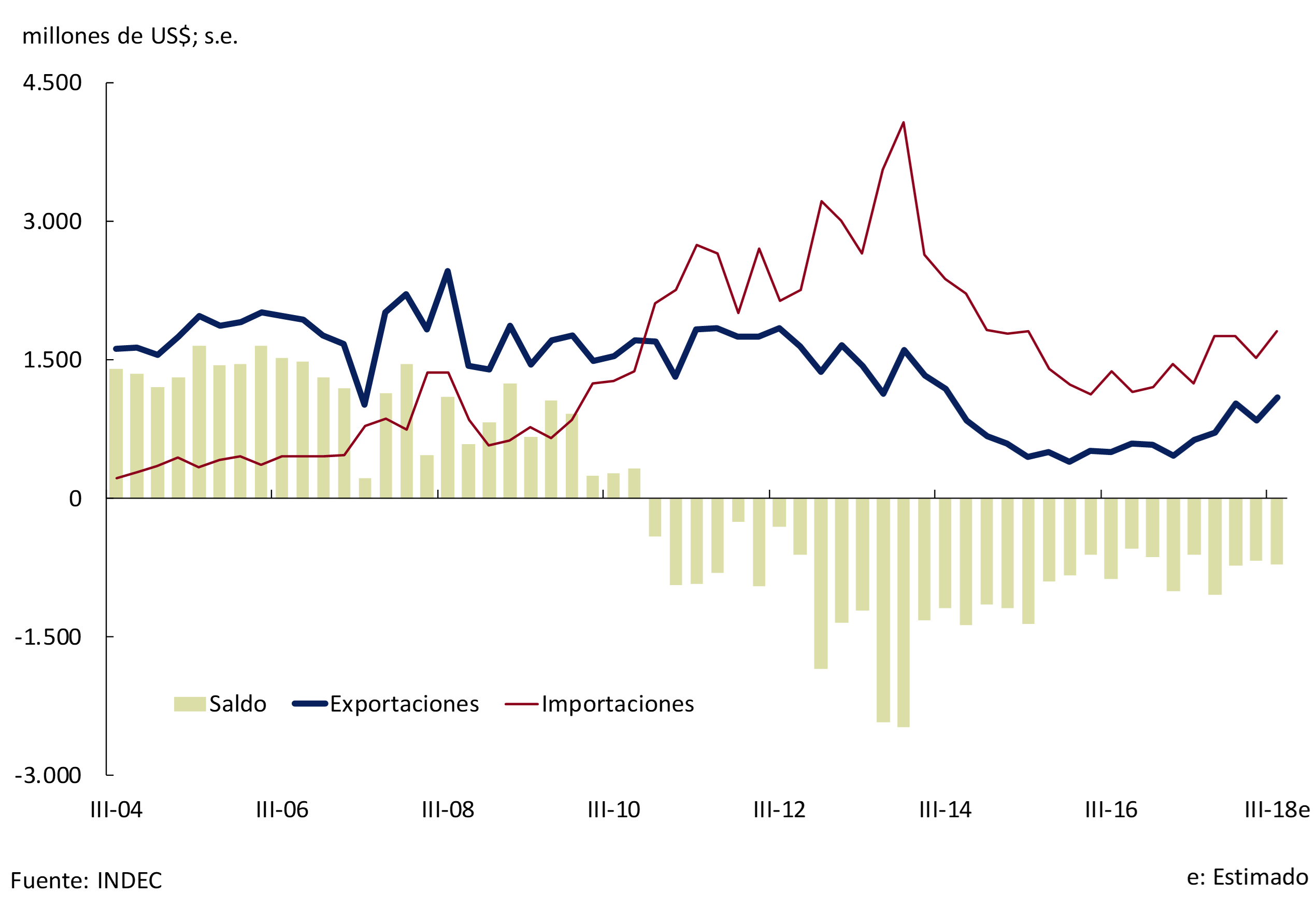
In addition to encouraging local gas production, energy policy faces important challenges such as expanding transmission and distribution networks, promoting a more efficient and sustainable use of each demanding group, and developing the great potential of renewable resources for electricity generation,48 with relative prices that are attractive for investments in the sector.
References
1 In October 2017 the ECB reduced its asset purchase programme from €60 billion per month to €30 billion, and from September of this year until the end of 2018 the pace of purchases slowed to €15 billion per month.
2 Unemployment rate not accelerating inflation.
3 The Target on the Federal Funds Rate.
4 According to the Commodity Price Index (CPI) published daily by the BCRA, which reflects the evolution of Argentina’s main export commodities.
5 A fall in the terms of trade has an unfavorable impact on Argentina’s trade balance, and an increase has a favorable impact.
6 In the October 2018 Global Financial Stability Report, the IMF analyzes the possible impacts of this tightening, concluding that emerging economies remain vulnerable, if this scenario comes to pass.
7 In the World Economic Outlook of October 2018, the IMF performs in Scenario Box 1. Global Trade Tensions (page 33) an analysis of the possible global impact of these measures. The Box concludes that there would be a loss of global GDP of 0.4% in the long term, in the most adverse scenario of all, if it were to occur.
8 The purpose of this indicator is to anticipate the turning points of activity from a recessionary to an expansionary phase or vice versa. On this occasion, the ILA had a turning point in November 2017 and the maximum in the “non-agricultural” EMAE was recorded a few months later, in April 2018. For more details, see Section 3/ BCRA’s Leading Index of Economic Activity, IPOM, January 2017.
9 According to the National Secretariat of Agroindustry, soybean production in the 2017/18 campaign fell 31.3% YoY and corn production fell 12.5%.
10 Monthly frequency index that includes traditional and non-traditional indicators of the consumption of goods and services. For more details see Section 1/ Private consumption, a variable difficult to follow in real time, IPOM July 2017.
11 The quarterly variations of the IBIF-BCRA indicator are a weighted average of the seasonally adjusted quarterly variations of the ISAC (INDEC), imports of capital goods (INDEC) and national production of capital goods (FIEL). The weights correspond to the weight of construction, investment in imported durable production equipment (EDP) and national EDP in the IBIF of the previous quarter. Between July and August, the ISAC fell 2.3% s.e. compared to the second quarter, imports of capital goods decreased 4.4% s.e. while the national production of capital goods increased 2.7% s.e.
12 Based on the monthly indices of quantities (2004=100) of the INDEC.
13 According to data from the Chamber of Industry and Commerce of Meat and Derivatives of the Argentine Republic (CICCRA), beef exports in tons of bone-in beef increased 72.6% y.o.y. in the first nine months of the year.
14 See Gervais, O. et al. (2016): “Current account dynamics, real exchange rate adjustment, and the exchange rate regime in emerging-market economies”.
15 Measured at basic prices.
16 Seasonally adjusted variation of July-August with respect to the second quarter of the Synthetic Indicator of Construction Activity (ISAC, INDEC). The Construya Index contracted 5.6% s.e. in the third quarter.
17 They begin by not replacing the personnel who leave the company (due to resignation, retirement, termination of contract, etc.).
18 The number of respondents who expect decreases in their staffing in the next 3 months practically equaled the number of employers who expect increases.
19 In the gas sector, projects are focused on increasing transportation and distribution. In electricity, investments are being promoted to expand the generation park, transport and distribution.
20 Between August 2016 and August 2018, beef production accumulated an increase of 17.2% driven by exports (data from the EMI of INDEC).
21 It should be noted that the wholesale basket has a smaller component of services than retail goods, so it is expected that the former will increase more than the latter in the face of an exchange rate shock.
22 Monetary aggregate over which the BCRA has the greatest control.
23 Calculated as the standard deviation relative to the mean of the responses for each period.
24 For more details on the first agreement signed with the IMF in June of this year, see the IPOM of July 2018.
25 For more details, see Communications “A” 6550, “A” 6556 and “A” 6569, respectively.
26 Until December 2016, the reference interest rate was the interest rate of the LEBAC with a 35-day term. From January 2, 2017 to May 2, 2018, it switched to the center of the interest rate corridor of 7-day term passes. As of August 8, 2018, it became the interest rate of the Liquidity Bills (LELIQ). Finally, as of October 1, 2018, the reference rate was defined as the average rate resulting from LELIQ’s daily operations with financial institutions.
27 It was also defined that banking entities could only participate in the primary LEBAC tenders on behalf of non-bank third parties, and could not sell their remaining LEBACs on the secondary market to non-banking entities.
28 For an analysis of the relationship between money and inflation in the world, see: McCandless, G. and W. Weber (1995). “Some Monetary Facts”. Quarterly Review. Federal Reserve Bank of Minneapolis. For an analysis of money and inflation in Argentina, see: Basco, E., L. D’Amato and L. Garegnani (2006). “Monetary Growth and Inflation: Argentina 1970-2005”. Working paper 2006/13. Central Bank of the Argentine Republic.
29 To see the effect of the level of the inflation rate on the relationship between money and inflation in Argentina, see: Basco, D’Amato and Garegnani (2006), and Teles, P. and H. Uhlig (2013). “Is Quantity Theory Still Alive?”. Working Paper No. 1605. European Central Bank.
30 For an analysis of the use of monetary aggregates in developed countries, see: Bernanke, B., and F. Mishkin (1992). “Central Bank Behavior and the Strategy of Monetary Policy: Observations from Six Industrialized Countries”. In Olivier Blanchard and Stanley Fischer, eds., NBER Macroeconomics Annual, Cambridge, MA: MIT Press, 183-238.
31 In LELIQ auctions, the Central Bank announces a tentative amount and the minimum placement rate. Once the bids are received, the monetary authority determines the cut-off rate and awards with multiple prices.
32 In addition, the rate of active passes was defined on a daily basis, resulting from multiplying a coefficient between 1.01 and 1.5 with the maximum rate paid by the current LELIQs, while the rate of passive passes became the result of multiplying a coefficient between 0.5 and 0.99 by the minimum rate announced for the LELIQs in force. For more details, see Communication “A” 6576.
33 For the multilateral real exchange rate corresponding to the upper and lower limits of the non-intervention zone, the values announced for October 1 of $34 and $44 per dollar adjusted to 3% per month until October 19 were considered.
34 These concepts correspond to those of “net importers and others in the real sector” and “natural persons” in the exchange statistics prepared by the Central Bank (see the BCRA’s report on the Evolution of the Exchange Market and Exchange Balance).
35 As an additional measure to encourage the collection of fixed-term deposits, institutions were allowed to pay interest at least 30 days, instead of paying in full at the end, which was the only one allowed by the previous rule. At the same time, the Central Bank decided to reduce the minimum daily minimum cash position to allow banks to participate more actively in the LELIQ auction operations to which the monetary authority convenes and thus cushion the effect of the monetary base target on the variability of the monetary policy rate. Finally, it allowed entities to acquire BCRA Cash Clearing Notes with part of their banknote holdings not affected by the “Interbank Banknote Clearing”, with an interest rate of 1/5 of the Central Bank’s reference rate. For more details, see Communication “A” 6575.
36 The BADLAR rate corresponds to deposits of more than $1 million arranged with a term of 30-35 days, while the TM20 corresponds to deposits of more than $20 million with a term of 30-35 days.
37 Ample liquidity: current account deposits at the Central Bank, cash, LELIQ, LEBAC, net passes and integration with the 2020 Bond.
38 Argentina is the second largest market for Bolivian gas after Brazil. According to the current contract, the state-owned company Yacimientos Petrolíferos Fiscales Bolivianos (YPFB), must send a minimum volume of 20.9 million m3 per day in the winter (between May and October) and 17.2 million m3 per day in the summer season.
39 This year the Government will not renew the contract with the regasification ship moored in the port of Bahía Blanca, which had been operating since 2008. The price that the state-owned company IEASA (Argentine Energy Integration, product of the merger of ENARSA with Emprendimientos Energéticos Binacionales S.A.) pays for imported LNG is variable and depends on each tender. Including transportation costs, at present around US$7/MMBTU is paid.
40 “Energy Subsidies, Devaluation and Prices”, Fernando Navajas, Working Paper No. 122, FIEL.
41 Carried out by IEASA and Compañía Administradora del Mercado Mayorista Eléctrico (CAMMESA) for electricity generators.
42 Through the Program to Stimulate the Surplus Injection of Natural Gas (Resolution 1/2013), the Government ensured a price of US$7.5/MMBTU for any type of gas – conventional, tight, shale and off-shore – injected into the domestic market above the base injection of each company. As of 2017, the Program only reaches unconventional investment projects and the way of accounting for subsidized production and penalties for non-compliance was modified (Resolution E 46/2017). A minimum price of US$7.50/MMBTU in 2018, US$7.00/MMBTU in 2019, US$6.50/MMBTU in 2020 and US$6.00/MMBTU in 2021 is assured.
43 Unconventional gas production currently accounts for about 25% of total production.
44 Energy imports are computed in tonnes of oil equivalent (TOE) to homogenise the units (source: Energy Balances 2014 and 2017).
45 The government authorized the companies Total Austral, Pan American Sur and Compañía General de Combustible to sell up to a total volume of 479.5 million m3 to the Chilean company Methanex, until June 1, 2020 (Resolution 104/2018).
46 CAMMESA began to dispatch electricity to the Brazilian firm ONS (600 MW of power).
47 For more details, see documents from the Ministry of Energy “Energy Scenarios 2030”.
48 In this sense, in December 2017 the Distributed Generation Law (27.424) was enacted, which allows residential and commercial electricity users to generate and inject their own energy from renewable sources into the grid.
Glossary
€: Euro
Acum.: Cumulative
AFCP: Portland Cement Manufacturers Association
AFIP: Federal Administration of Public Revenues
AUH: Universal Child Allowance for Social Protection
BADLAR: Buenos Aires Deposits of Large Amount Rate (interest rate paid for fixed-term deposits of more than one million pesos in the 30 to 35-day bracket by the average of banking entities)
BCB: Central Bank of Brazil
BCBA: Buenos Aires Stock Exchange
ECB: European Central Bank
BCRA: Central Bank of the Argentine Republic
BONAR: Argentine Nation Bond
CABA: Autonomous City of Buenos Aires
CEMBI+: Corporate Emerging Market Bond Index Plus
CEMBI+AR: Corporate Emerging Market Bond Index Plus Argentina
ECLAC: Economic Commission for Latin America and the Caribbean
CER: Reference Stabilization Coefficient
FIGURE: Research and Training Center of the Argentine Republic – Central de Trabajadores de la Argentina (CTA)
COICOP: Classification of Individual Consumption According to Purpose
CNV: National Securities Commission
Contrib.: Contribution
S Fuels Energy
DJVE: Affidavits of Foreign Sales
e: Dear
EDP: Durable Production Equipment
EIL: Survey of Labor Indicators
EMAE: Monthly Estimator of Economic Activity
EMBI+: Emerging Markets Bond Index Plus
EMBI+AR: Emerging Markets Bond Index Plus Argentina
EMBIG: Emerging Market Bond Index Global
ENGHo: National Survey of Household Expenditure and Income
EPH: Permanent Household Survey
excl.: Excluding
Fed: Federal Reserve of the United States
FIEL: Latin American Economic Research Foundation
IMF: International Monetary Fund
IMF WEO: World Economic Outlook
FOB: Free on Board (purchase and sale operations carried out by boat)
FOMC: Federal Open Market Committee
GBA: Greater Buenos Aires
A.I.: Year-on-year
IAMC: Argentine Institute of Capital Markets
IBIF: Gross Domestic Fixed Investment
ICC: Consumer Confidence Index prepared by the Torcuato Di Tella University
ICC-INDEC: Construction Cost Index
IGA-OJF: Orlando J. Ferreres General Activity Index
ILA: Leading Activity Index
ILCO: BCRA’s Leading Indicator of Private Consumption
INDEC: National Institute of Statistics and Censuses
INML: Liniers Market Steer Index
CPI: Consumer Price Index of national coverage released by INDEC
IPCBA: Consumer Price Index of the City of Buenos Aires
CPI Cordoba: Consumer Price Index for the Province of Cordoba
CPI GBA: Consumer Price Index of Greater Buenos Aires
CPI-NP: Weighted National Indicator
CPI San Luis: Consumer Price Index of the Province of San Luis
IPIB: Basic Domestic Price Index
IPIM: Internal Wholesale Price Index
MPPI: Commodity Price Index
IPOM: Monetary Policy Report
ITCNM: Multilateral Nominal Exchange Rate Index
ITCRM: Multilateral Real Exchange Rate Index
VAT: Value Added Tax
kg: Kg
LAC: Latin American Consensus Forecasts
LEBAC: Central Bank Bills (Argentina)
LELIQ: Liquidity Bills of the Central Bank of the Argentine Republic
LFPIF: Financing Line for Production and Financial Inclusion
M2: Banknotes and coins + quasi-currencies in circulation + current accounts in $ and savings accounts in $
Mens.: monthly
MERVAL: Buenos Aires Stock Exchange
mill.: Million
Min.: Ministry
IPM: Input-output matrix
MOA: Manufactures of Agricultural Origin
MOI: Manufactures of Industrial Origin
MRO: Main refinancing operations
MSCI: Morgan Stanley Capital International Index
MULC: Single and Free Exchange Market
NEA: Northeast Argentina
NG: General level
NOA: Northwest Argentina
OECD: Organisation for Economic Co-operation and Development
OPEC: Petroleum Exporting Countries
bp: Basic points
p.p.: Percentage points
p: Projected
PAMI: Social Work for Retirees and Pensioners
PCE: Personal consumption expenditures
PCP-BCRA: Contemporary BCRA GDP Prediction
EAP: Economically Active Population
GDP: Gross Domestic Product
PMI: Purchasing Managers’ Index
PP: Primary Products
Prom. Moving Average: Moving Average
Avg.: Average
R$: Real
REM: BCRA Market Expectations Survey
REPO: Repurchase Agreement (Operación de Recompra)
ROE: Records of Export Operations
REPO Round: Average interest rate of 1-business day transactions between financial institutions in the guaranteed market
S.A: Sociedad Anónima
s.e.: Series without seasonality
SSPM: Private Consumption Indicator prepared by the Ministry of Finance
TFF: Federal Funds Rate
tonnes: tonnes
TN: National Treasury
APR: Annual Nominal Rate
Trim.: Quarterly / Quarter
ICU: Utilization of installed capacity
US$: US Dollars
UTDT: Universidad Torcuato Di Tella
UVA: Unit of Purchasing Value
Var.: Variation
Vol.: Volume
YPF SA: Yacimientos Petrolíferos Fiscales Sociedad Anónima


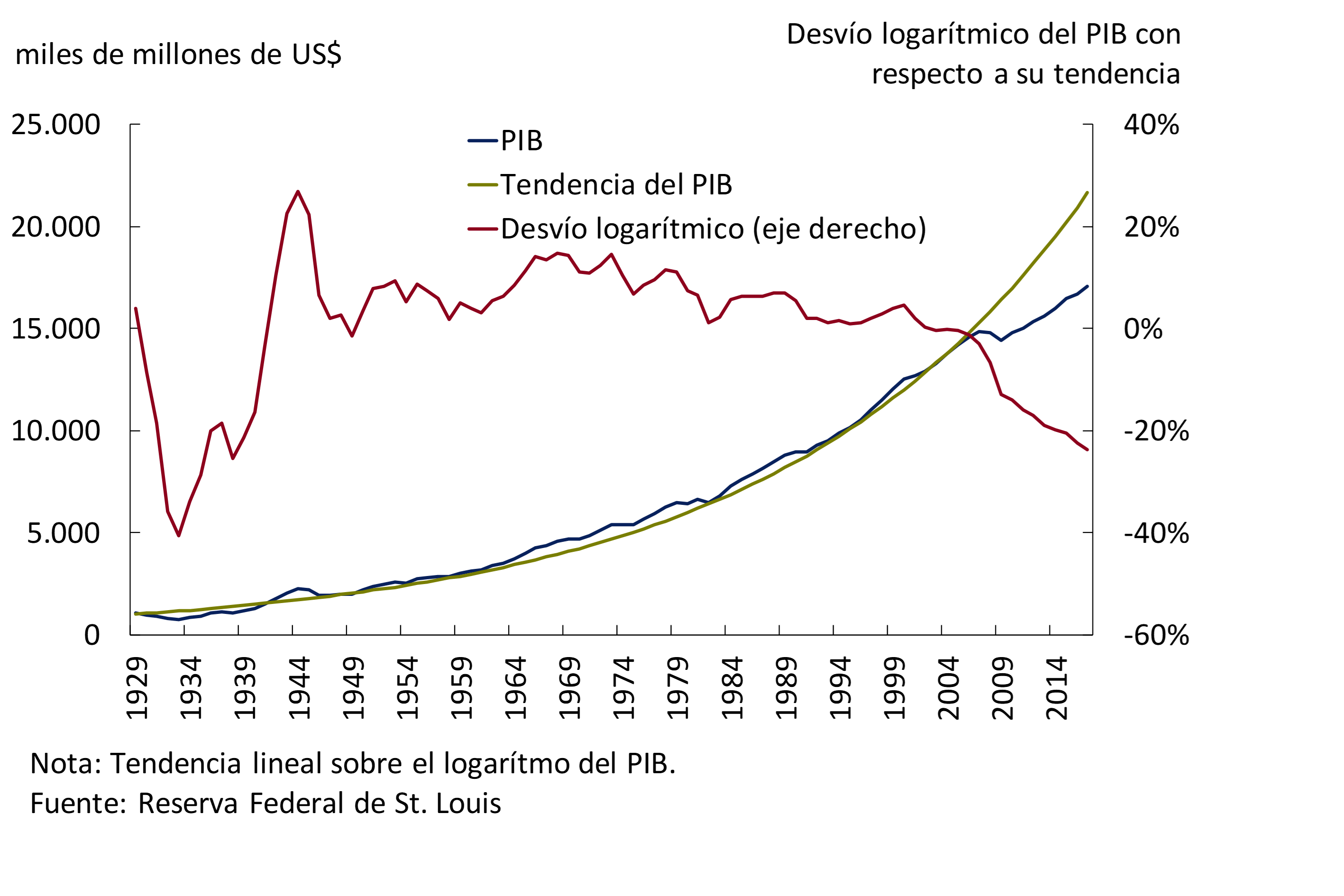