1. Monetary policy: assessment and outlook
Since October 2018, the Central Bank of the Argentine Republic has been carrying out a scheme based on strict control of the monetary base and the definition of an exchange rate reference zone (formerly called the foreign exchange non-intervention zone). During the second quarter of the year, the Central Bank continued to meet its goal of zero growth of the monetary base (WB) every month, which remained at $ 1,343.2 billion.
The monetary aggregate scheme reduced the nominal volatility recorded until the third quarter of last year, and inflation began to decline from the peak of 6.5% per month recorded in September 2018. However, during the first quarter of 2019, the concentration of increases in regulated prices, to which were added the lagged effects of the exchange rate depreciation of 2018 and a new episode of exchange rate volatility, caused inflation to rise again.
Faced with this situation, the Monetary Policy Committee (COPOM) took a series of additional measures during March and April 2019 to strengthen the monetary-exchange rate scheme: 1) it reduced the monetary base target by $43 billion, eliminated the seasonal adjustment of the target set for June and extended the commitment to zero growth of the monetary base to all of 2019, initially planned until June 2019; 2) established a minimum reference interest rate; (3) set the growth of the limits of the exchange reference zone at zero, leaving the upper limit constant at 51.448 pesos per dollar and the lower limit at 39.755 pesos per dollar until the end of the year, and decided to refrain from buying foreign currency if the exchange rate was below the reference zone; and 4) it provided that foreign currency sales may be made in the foreign exchange market in the event of episodes of excessive volatility, even if the exchange rate is within the reference zone (see section 3).
The measures adopted and the maintenance of a contractionary monetary policy, in a context of better international conditions, stabilized the foreign exchange market and inflation expectations, allowing inflation to resume its downward path since April. This in turn led, together with a series of measures implemented by the Executive Branch to shore up household spending, that economic activity continued with the recovery that began in December.
In an environment of lower nominal volatility and falling inflation expectations, the nominal interest rate of the LELIQ showed a downward trend since the beginning of May, reaching the minimum level of 62.5% that had been established since April and until the end of June. To guarantee the contractionary bias of its monetary policy, and in a cautious attitude in the face of possible episodes of uncertainty, the COPOM reduced the floor of the benchmark interest rate to 58% during July. This reduction recognizes that there has been a drop in inflation and inflation expectations in recent months, but at the same time recognizes that the economy is still going through a period of uncertainty. This ensures that the real interest rate remains at positive high levels.
Additionally, to promote competition among financial institutions and improve the mechanism for transmitting the reference rate to the interest rates received by savers, the Central Bank allowed bank customers to make fixed-term deposits in pesos online at any financial institution without the need to be a customer or carry out additional procedures. In this way, retail fixed-term interest rates grew and approached those of larger transactions (see section 5).
The fulfillment of the goal is particularly demanding in the months of June and July, due to the seasonal behavior of the demand for BM, which increases due to the payment of the half bonus and the higher expenses of the winter recess. In order to allow for better management of liquidity conditions during this period, the BCRA decided to establish a joint reserve position for the months of July-August, and for the months of December-January, where a similar phenomenon is repeated (see section 4).
In addition, and to also contribute to strengthening the transmission of the interest rate of the LELIQ, it was decided to reduce by 3 p.p. the minimum cash requirement on fixed-term deposits as of July. This represents a reduction in the demand for the monetary base due to reserve requirements of approximately $45 billion that compensates for the seasonal increase in demand per working capital. In order not to relax monetary policy, once this seasonal phenomenon has been overcome, the monetary base target will be reduced as of August to reach $1,298.2 billion in October, fully offsetting the effect of the reduction in reserve requirements.
The BCRA’s view is that the macroeconomic conditions are in place to achieve sustainable disinflation, given that basic macroeconomic balances have been restored. Fiscal balance is being achieved and monetary financing from the Treasury has ceased. The exchange rate today is competitive, with a level in June that is around 50% higher than the value recorded prior to the exchange rate unification of December 2015, which has made it possible to correct the imbalance of the external sector. In addition, distortions generated by energy price arrears have been virtually eliminated. In turn, the BCRA has a strengthened balance sheet, with a sustainable level of interest-bearing liabilities and an adequate stock of international reserves, along with greater degrees of freedom to intervene in the foreign exchange market.
However, disinflation processes tend to be gradual and not linear, given that monetary policy operates with lags, and inflation also has an inertial component. This inertial component is reinforced after more than a decade of high inflation. Thus, the contractionary bias of the monetary scheme will remain throughout 2019, and the benchmark interest rate is expected to fall gradually and only as inflation falls. However, this medium-term trend could be temporarily disrupted in the event that some of the risks to which the economy is exposed materialize, such as a new episode of volatility in global financial conditions, or the usual uncertainty of electoral processes. In the current scheme, the endogenous interest rate allows us to respond immediately to any unforeseen shock.
Therefore, the BCRA must be persevering in its policy of strict control of the quantity of money and thus achieve a lasting reduction in inflation, providing an environment of stability conducive to economic growth.
2. International context
So far in 2019, the slowdown in the level of global activity that had begun to be observed at the end of 2018 continued, now extended to the main developed and emerging economies. As a result, the expected growth for Argentina’s main trading partners went from being the highest in the last six years in January of this year (2.2% average expected for 2019), to being the lowest in the last four years (1.2% average expected for the same period) according to the most recent projections. This is mainly due to the sharp decline in growth projections for Brazil.
Monetary authorities in advanced economies are responding to this scenario with a more expansionary policy path. Something similar is observed in most emerging countries. In this context, it is feasible that global liquidity conditions for emerging markets will continue to improve, as long as the effect of uncertainty related to trade and geopolitical tensions is not greater, and that this leads to a flight to quality.
Therefore, a mixed international scenario continues to be observed for Argentina. On the one hand, lower global growth prospects in general, and in particular, for the country’s main trading partners. On the other hand, the conditions are in place for a better external financial scenario, as long as the current stress factors are not strengthened, and therefore a capital outflow from emerging countries to the main advanced countries is triggered. Precisely, the main risk factor in the international context would be that trade disputes between the United States and China deepen (see Section 1).
2.1 There was a deterioration in the level of global activity that had a negative impact on the main trading partners, which would lead to expansionary monetary policies in some of these countries
Signs of slowdown in global economic activity continued in recent months. 1 The most recent global trade data evolved in this regard, falling by 2.3% s.e. from the peak of October 2018, while industrial production fell by 0.2% s.e. in the same period (see Figure 2.1).
Figure 2.1 | Global trade and industrial production volume
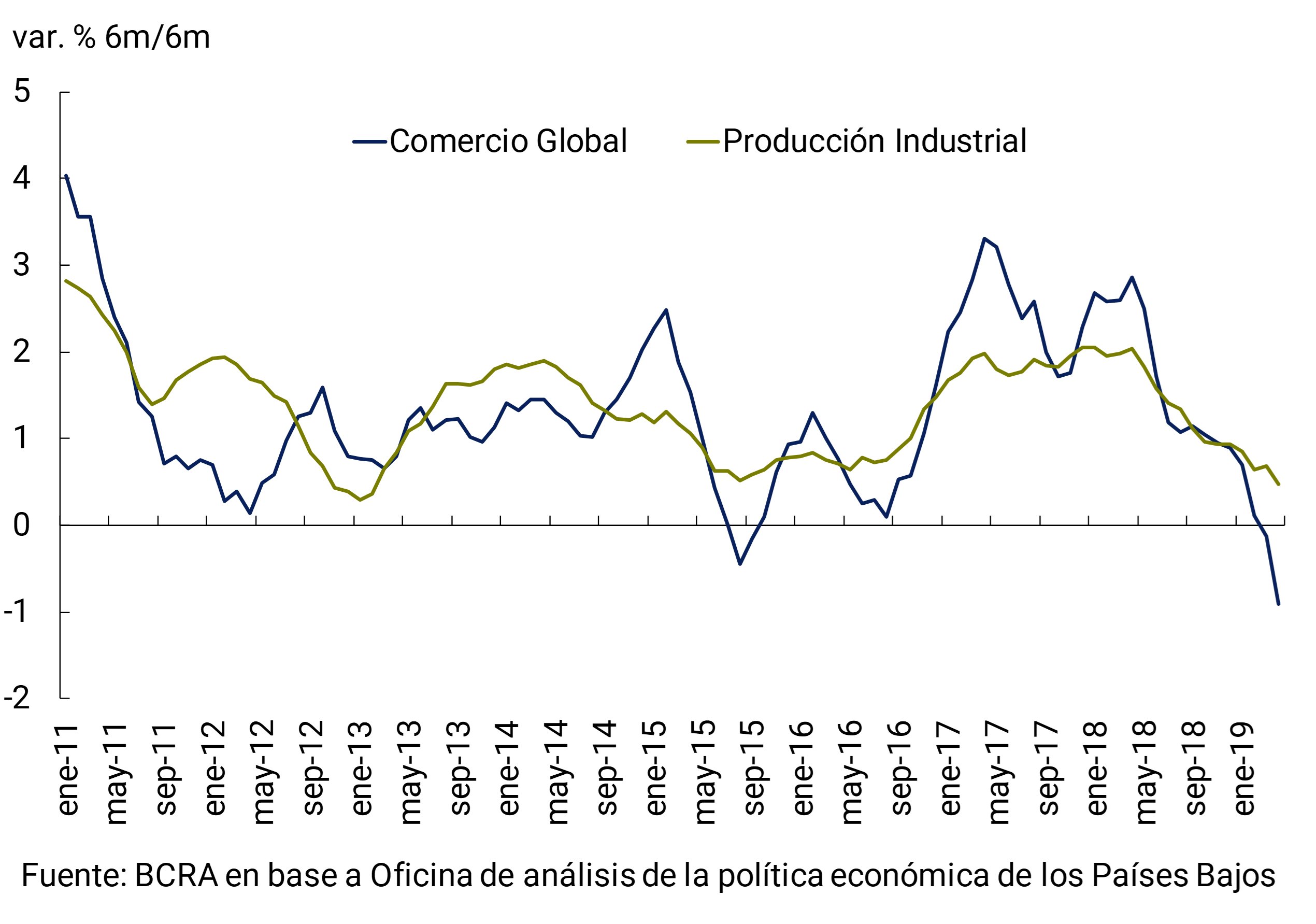
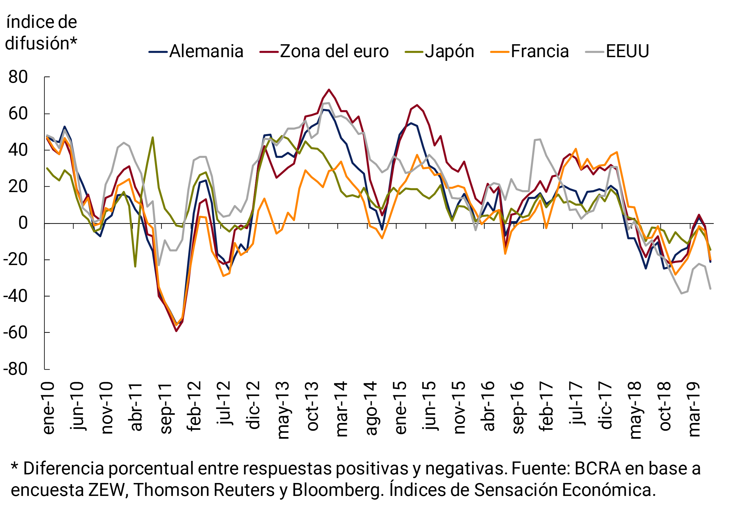
As mentioned in the previous IPOM, a considerable part of the decline in the pace of global growth would appear to be linked to a marked reduction in capital goods investment. This lower investment could be explained by the uncertainty generated by trade tensions and their impact on business confidence (see Figure 2.2).
Figure 2.2 | Economic Expectations in Advanced Economies
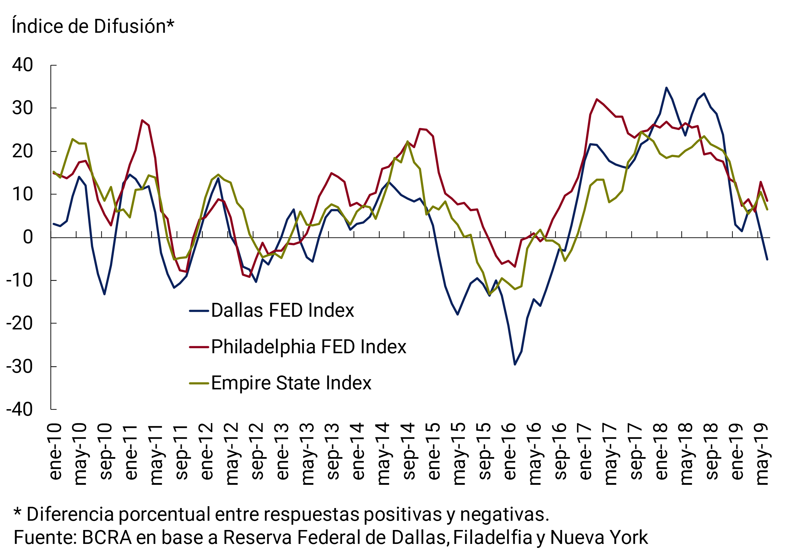
This is reflected in most of the manufacturing PMI indices that in the previous IPOM were in the expansion zone, and became in the contraction zone. Something similar happens with the global PMI of the industry (see Figure 2.3). The overall PMI for the services sector, although still in the expansion zone, has a clear trend towards the contraction zone, the same is true for the composite PMI. On the other hand, inflation rates in the main advanced economies (the United States, the euro area, Japan and the United Kingdom) remain low in all cases, which gives the monetary authorities room to take measures with an expansionary bias.
Figure 2.3 | Global PMI indices

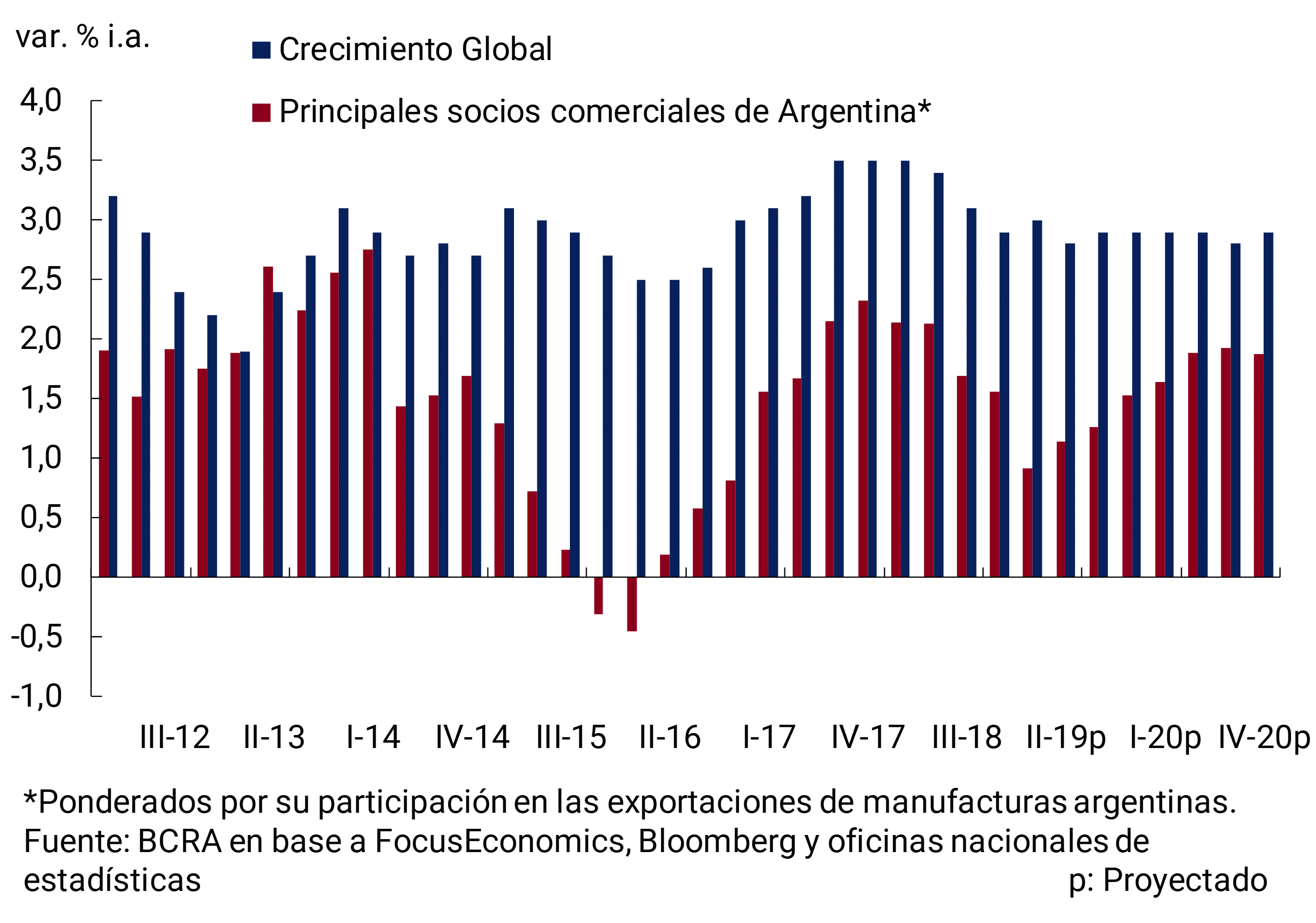
This panorama of lower global growth is also observed in the level of activity of Argentina’s main trading partners. For these countries, the expected growth for 2019, which until the IPOM of January of this year was the highest in the last six years, became the lowest in the last four years (see Figure 2.4). However, the negative impact on Argentina of Brazil’s expected lower growth could be partially offset by more competitive levels of real exchange rates.
Figure 2.4 | Growth of Argentina’s trading partners
Much of the decline in growth expectations for our trading partners is linked to Brazil’s expected poorer performance. Growth in this country was negative in the first quarter by 0.2% s.e. (compared to the previous quarter) mainly due to the performance of investment and exports. In the same sense, the monthly activity data measured by the IBC-Br estimator of the Central Bank of Brazil (BCB) showed negative rates of variation in the first four months of the year. On the other hand, the most recent estimates of the BCB’s Focus survey foresee growth for 2019 of 0.8% YoY, 1.2 p.p. lower than the growth forecast in April. Lower external demand due to the expected lower level of global activity, local political uncertainties, and fiscal reforms are factors that negatively impact Brazilian growth in 2019.
In this regard, and as in the previous IPOM, an unfavorable change in investors’ perception of the structural reform process continues to be a potential destabilizing risk factor for the Brazilian economy. Thus, the BCB in its latest Inflation Report highlights the importance that progress in the structural reform agenda would have in Brazil’s economic performance for this year. Therefore, the BCB forecasts GDP growth in 2019 of 0.8% YoY, but conditional on progress being made in this regard.
Figure 2.5 | Brazil. Macroeconomic indicators
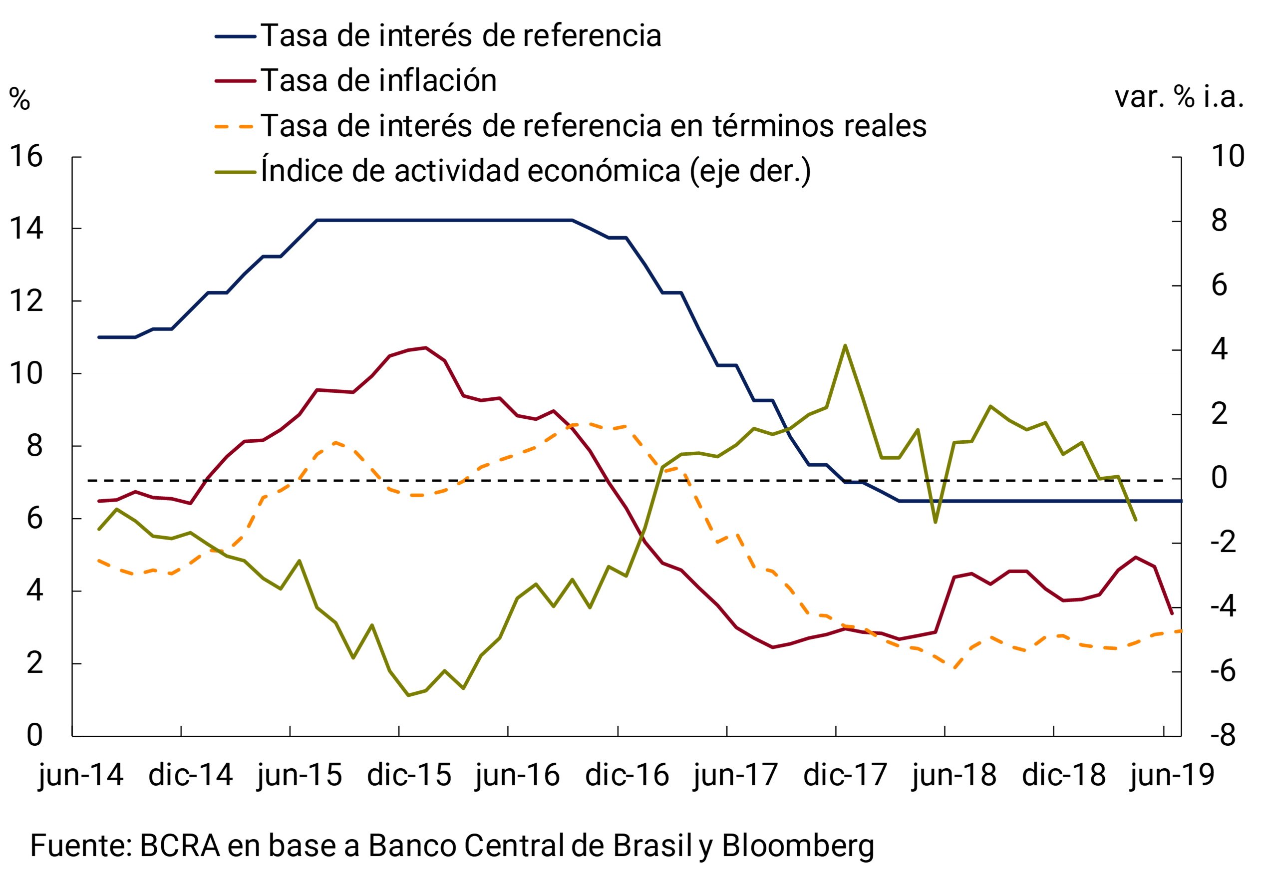
The most recent inflation data in Brazil (June) was 3.4% year-on-year, below the center of the target (4.25% ± 1.5). Inflation in the first months of the year was driven by specific factors that have lost strength since mid-2019. In turn, analysts surveyed by Focus predict that the inflation rate will end 2019 at 3.8%. The BCB recently left the monetary policy interest rate (SELIC) unchanged, which has been at 6.5% since the end of March 2018 (see Figure 2.5). Unlike the previous IPOM, where no changes were expected, in the latest Focus analysts project a reduction of 1 p.p. by the end of the year. The main reasons that would lead to reducing the target on the SELIC rate would be inflation below the target, lower growth prospects in Brazil and in the world, together with the increasingly likely expansionary monetary policy measures of the main central banks.
Figure 2.6 | U.S. Consumer Expectations

The most recent data on activity in the United States show that GDP grew in the first quarter by 3.1% (compared to the previous quarter, seasonally and annualized), more than 0.2 p.p. above the market consensus, and 0.9 p.p. more than the previous quarter. In a context where GDP grew in the last year at a rate of 3.2% on average, the indications that the United States Federal Reserve (Fed) would reduce its benchmark interest rate in 2019 are explained by several factors. Among these: 1) the aforementioned deterioration in the level of world activity; (2) the slowdown in the rate of increase in hourly pay; 3) the inflation rate (measured by the core deflator of household spending) has been below or around the target since mid-2012; and 4) the evolution of different indicators that in other economic cycles functioned as predictors of recession (see Figures 2.6, 2.7 and 2.8).
Figure 2.7 | Unemployment rate and employment differential in the United States

The Fed lowered its policy interest rate projections. In December 2018, an increase of 0.5 p.p. was expected during 2019, while in the latest projections it is expected to remain unchanged during the year. But, as mentioned, there are indications (including statements by Fed authorities) about the growing possibility of a reduction in the same in the coming months. This change in such a short term could also be understood because, given the proximity to the effective lower bound (elb2) that reduces the margin for action of monetary policy, it would be advisable, in order to increase its effectiveness, to overreact to the first indications of the need for monetary stimulus (for more details see this conference). Finally, the projections for the rest of the economic variables released by the Fed at its June meeting remained almost unchanged, except for inflation, which decreased slightly compared to March.
Figure 2.8 | Business confidence level in regions of the United States
In the euro area, economic activity performed better than expected by the market consensus (0.3%) in the first quarter, with growth of 0.4% s.e. This would have been due to one-off factors, such as the UK’s exceptional demand for euro area goods (linked to possible Brexit). In addition, after the implementation of the Worldwide Harmonised Light Vehicle Test Procedures (WLTP)3 , an increase in vehicle procurement was observed – especially in Germany. On the other hand, there was higher private consumption in the quarter due to fiscal stimulus measures that came into force at the beginning of the year, and whose greatest impact would be concentrated in the first quarter. Finally, better weather conditions than in the previous quarter allowed an increase in construction activity in some countries.
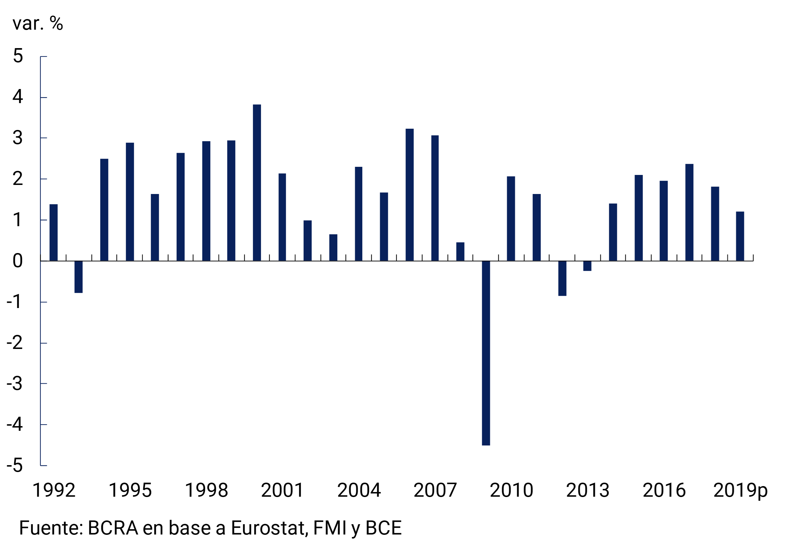
However, similar to the case of the United States monetary authority, the European Central Bank (ECB) also went from giving signals that it would be ready to increase its benchmark interest rate in 2019, to taking expansionary measures in April 2019 (see the IPOM of April 2019). and to signal in early June that it is ready to resort to new expansionary measures (probably a new quantitative easing program). Also, the ECB at its last meeting mentioned global factors with a direct impact on business confidence that would be markedly affecting the growth prospects of the euro area, which is being sustained mainly by private consumption. As a result, the growth rate projected by the ECB for this year (1.2% YoY) is the lowest in the last six years (see Figure 2.9).
Figure 2.9 | Euro area GDP growth
China’s economy continues to slow. After growing in 2018 at 6.6%, the lowest rate of expansion since 1990, in the first quarter4 of the year it registered a growth of 6.4% year-on-year. Moreover, according to the Focus Economics survey, analysts expect the growth rate to continue to slow until it stabilizes at around 6% by the end of 2020. Several factors converge to explain this slowdown: the effects of the imposition of mutual tariffs with the United States (see Section 1), the still failed attempt by the authorities to boost private consumption to the detriment of investment, and the credit deleveraging policies carried out until recently by the People’s Bank of China (PBOC, the monetary authority). Industrial production in general has been affected, with growth rates that are around seventeen year lows.
The Chinese authorities implemented some stimulus measures based on tax cuts and increased spending on public infrastructure, and put on hold the policies of deleveraging the financial system. In this regard, they have recently reduced the requirements for reserve requirements. At the end of May, in the face of serious credit risks, the PBOC and China’s bank and insurance regulatory commission took control of Baoshang Bank, announcing a restructuring aimed at cleaning up its balance sheet. The last time the Chinese authorities took such a measure was in 1998. In this context, the monetary authority has been injecting liquidity through open market operations, and could again reduce reserve requirements, in order to avoid problems in other financial institutions.
2.2 Global liquidity conditions for emerging markets are likely to improve
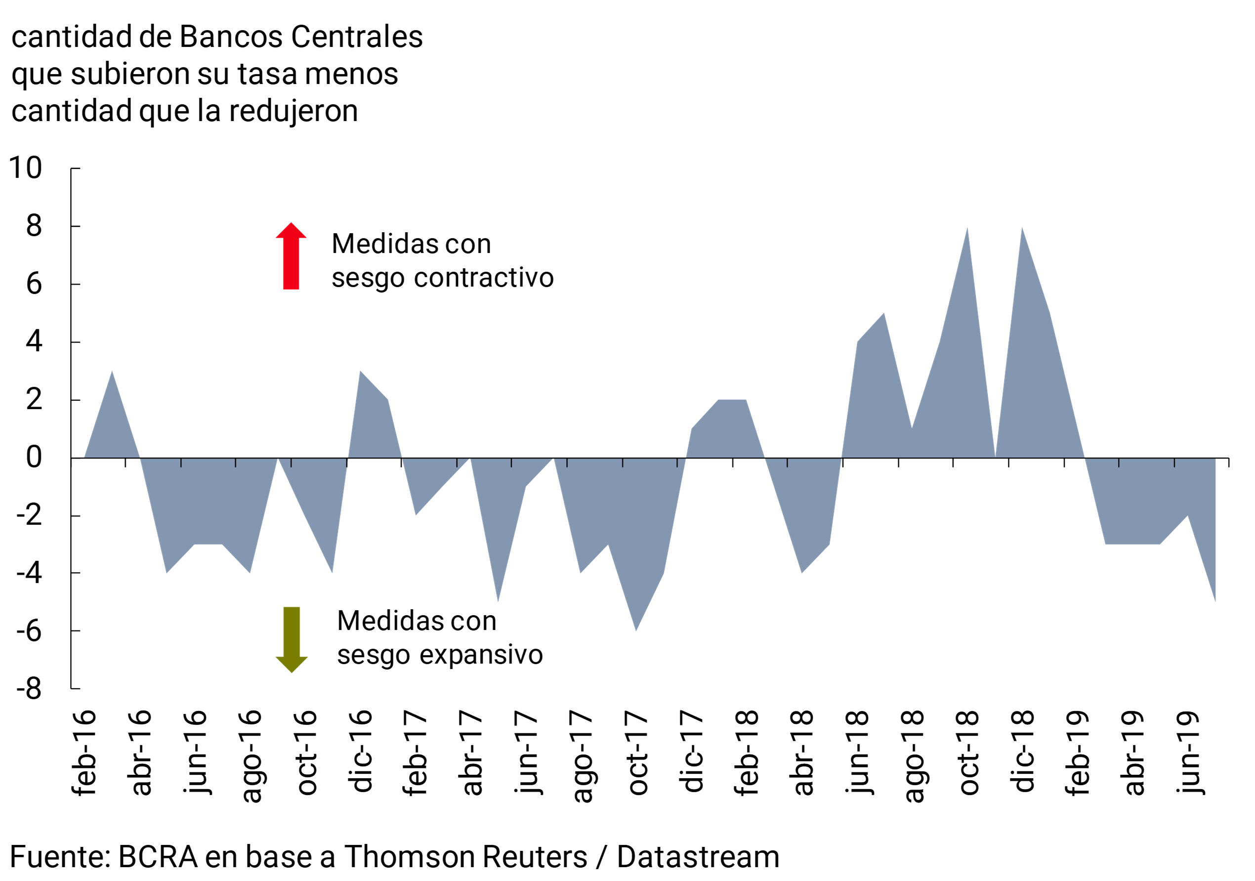
As mentioned, the monetary authorities of the largest economies would be about to implement monetary policies with an expansionary bias again. Something similar is observed in the case of emerging countries, where the bias of monetary policy would be leaning towards expansionary (see Figure 2.10). In this context, it is feasible that global liquidity conditions for emerging markets will improve, as long as the effect of uncertainty related to trade and geopolitical tensions that leads to a flight to quality process is not greater.
Figure 2.10 | Monetary Policy Tightening and Expansion Cycles
Sovereign and corporate risk premiums in emerging economies rose towards the end of the second quarter of 2019, after the decline experienced in the first quarter of the year, and remain at high levels compared to recent years. However, emerging market debt placements in international markets showed the first year-on-year increase in the second quarter of 2019 after four consecutive quarters of declines. The amount of gross placements (sovereign and corporate) increased 8% YoY in the second quarter (compared to a 7% YoY drop in the previous quarter). This was explained by the performance of the corporate segment (with an expansion of 35% YoY), while sovereign issuances contracted 40% YoY.
In this context, the yield differential required in the secondary markets for Argentine sovereign debt between peaks remained almost unchanged from the previous IPOM, at around 800 bps, having momentarily exceeded 1,000 points in early June, and then fell by more than 200 bps (see Figure 2.11). In the quarter there were no new international placements of the sovereign, because given the agreement with the International Monetary Fund and as it emerges from the Financial Program, the National Government has no need to access these markets in the remainder of 2019 and 2020.
Figure 2.11 | Sovereign and corporate debt risk indicators
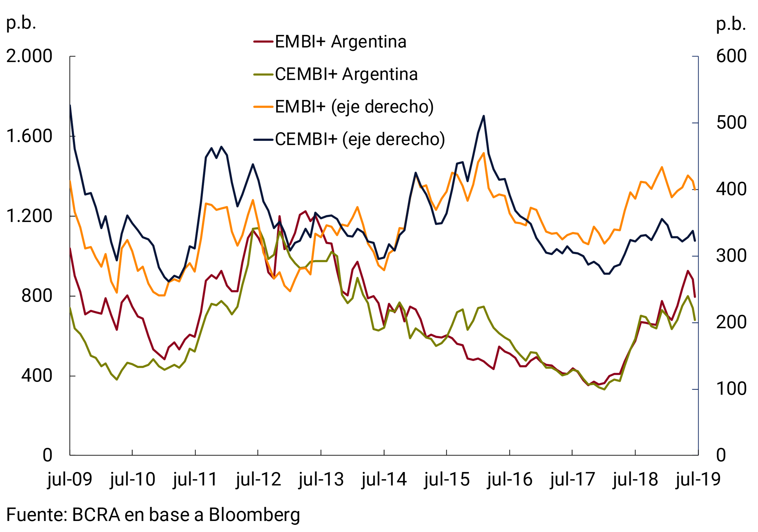
For its part, despite the fact that Argentina’s CEMBI behaved in a similar way to the sovereign index, there were some one-off placements of Argentine corporate debt in foreign markets by companies in the metallurgical and energy sectors. Placements by publicly offered companies in international markets in the second quarter of 2019 totaled US$650 million (one of which was made with a guarantee of export collections), while in the same period of 2018 there was a single placement at the end of April for US$500 million.
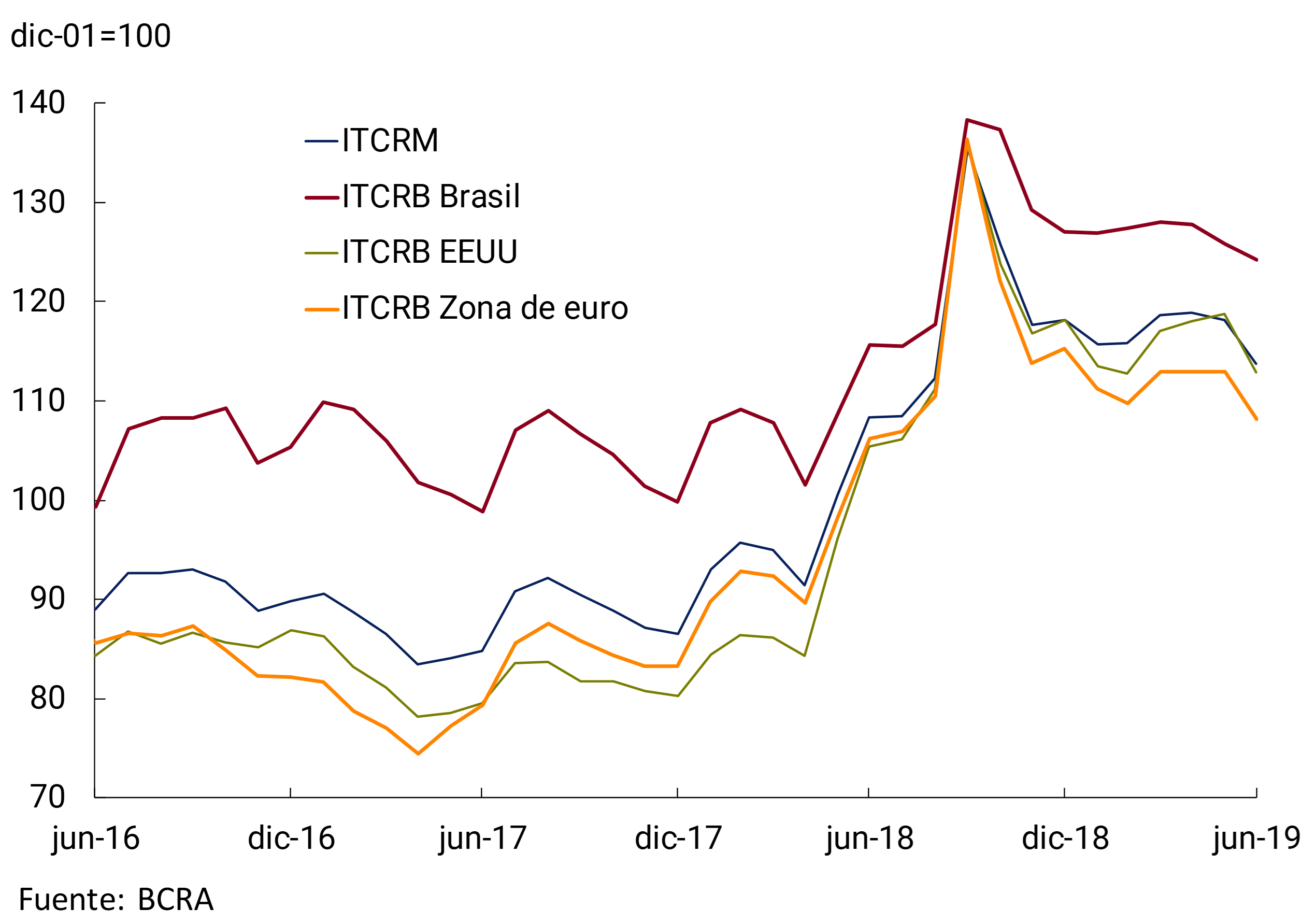
After registering a relatively stable evolution throughout the second quarter, the Multilateral Real Exchange Rate Index (ITCRM) fell in the last days of June. Thus, at the end of June it was around 8% below the level recorded at the beginning of April, and returned to levels close to those of August 2018. However, it is 51% above the value of November 2015 (see Figure 2.12). The evolution of the bilateral nominal exchange rate of the Argentine peso with the dollar accompanied the movement of the main Latin American currencies.
Figure 2.12 | Multilateral and bilateral real exchange rate
2.3 At the margin, the prices of Argentine agricultural exports improved slightly
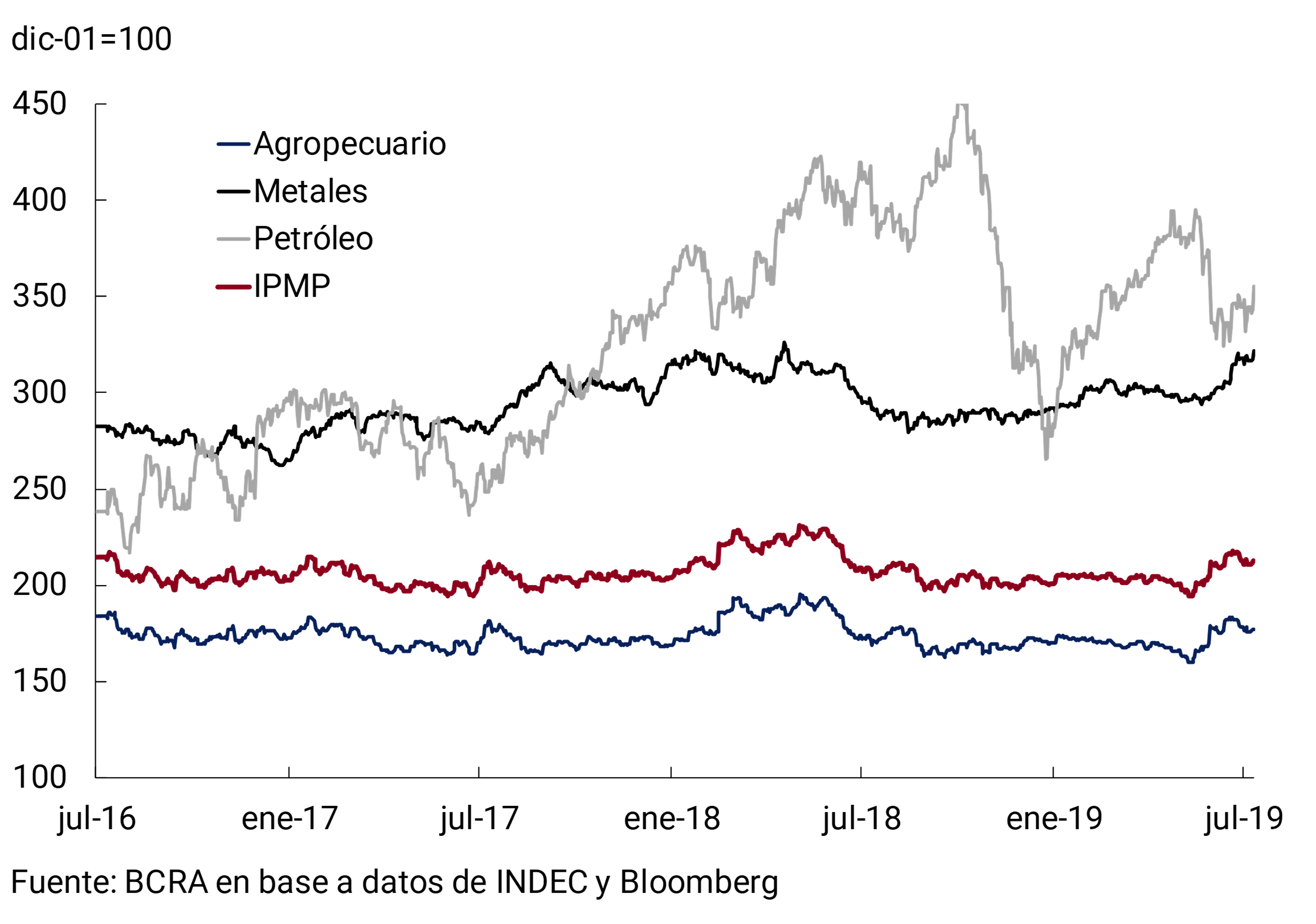
In the second quarter of the year, international commodity prices measured in dollar5 increased slightly compared to the previous quarter – mainly since the end of May – mainly due to the evolution of the grouping of agricultural raw materials and metals, while crude oil values fell at the margin. Since the end of May, international agricultural commodity values have been boosted by delayed U.S. corn and soybean planting due to excess soil moisture. In any case, during the second quarter, the prices of the main commodity groups remained on average below the levels they had in the same period of 2018, implying a 9% YoY drop in the Commodity Price Index (CPI), which reflects the evolution of Argentina’s main export commodities (see Figure 2.13).
Figure 2.13 | Commodity Price Index
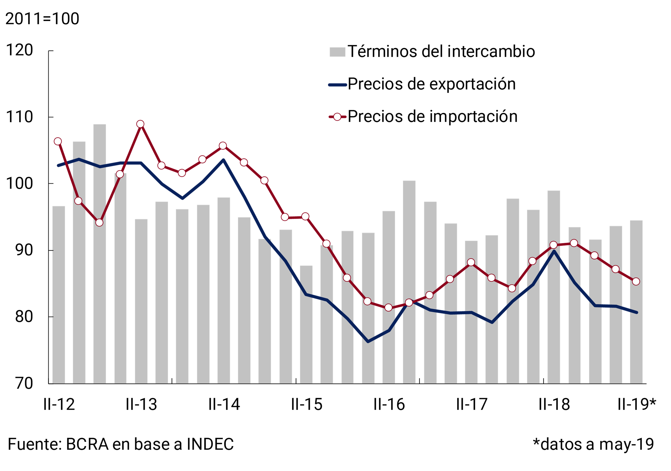
The data available for the April-May two-month period indicate that there was a 1.2% drop in Argentina’s export prices compared to the previous quarter, mainly due to the decrease in the quotations in dollars of primary products in that period (-6%). Meanwhile, import prices showed a 2.1% drop in the same period, with a strong incidence of reductions in the dollar prices of imported capital goods and their parts. As a result, the terms of trade rose slightly (0.9%) and remained around the average level of the last 3 years (see Figure 2.14). It is estimated that as of June, export prices would have begun to reflect higher international quotations for the main agricultural products.
Figure 2.14 | Terms of Exchange
In summary, the recent slowdown in the level of global activity was generalized to the major developed and emerging economies. In this context, both advanced and emerging economies are returning to a path of more expansionary monetary policies. This makes it feasible that global liquidity conditions for emerging markets will continue to improve, as long as the effect of uncertainty related to trade and geopolitical tensions is not greater, ending in a flight to quality. That is why the main risk factor in the international context continues to be the deepening of trade disputes between the United States and China.
3. Economic activity
During the second quarter, economic activity resumed the recovery that began in December, which had been temporarily interrupted in March. In addition to the positive impact on activity of the record agricultural harvest and the mobilization of resources associated with Vaca Muerta, there was an increase in consumer confidence. Domestic demand recovered in a context of better international financial conditions and lower exchange rate volatility. The REM estimates a 0.7% s.e. quarterly increase for the second quarter of 2019. The Leading Activity Index (ILA-BCRA) for May met all the necessary criteria to confirm that activity would enter an expansionary phase.
For the remainder of the year, private consumption will recover from the improvement in household incomes in combination with the programs implemented by the National Government that will tend to boost spending. At the sectoral level, the favorable performance of agriculture and gas and oil production is compounded by growth prospects in other activities that produce tradable goods and services based on a higher real exchange rate and the opening of new markets. The vision of a recovery of the economy is shared by REM analysts who project the beginning of an expansive phase during 2019 and growth for 2020.
3.1 During the second quarter, signs of recovery in the economy were evident
In the first quarter of 2019, GDP contracted 0.2% quarter-on-quarter and 5.8% compared to the same period of the previous year. The result was in line with what was forecast by market analysts at the REM in May and below what was expected in the latest Contemporary GDP Prediction (0.5% s.e; PCP-BCRA). The slight contraction in the first quarter was explained by a sharp temporary drop in activity in March, associated with greater exchange rate volatility, which interrupted the recovery that had begun in December.
During the second quarter, the BCRA introduced some modifications to the monetary-exchange regime (see Monetary Policy Chapter) that contributed to reducing exchange rate volatility and improving financial conditions. In this context of less uncertainty, the Executive Branch implemented a series of measures towards the end of April that underpinned household spending, the impact of which will last beyond the second quarter (see box).
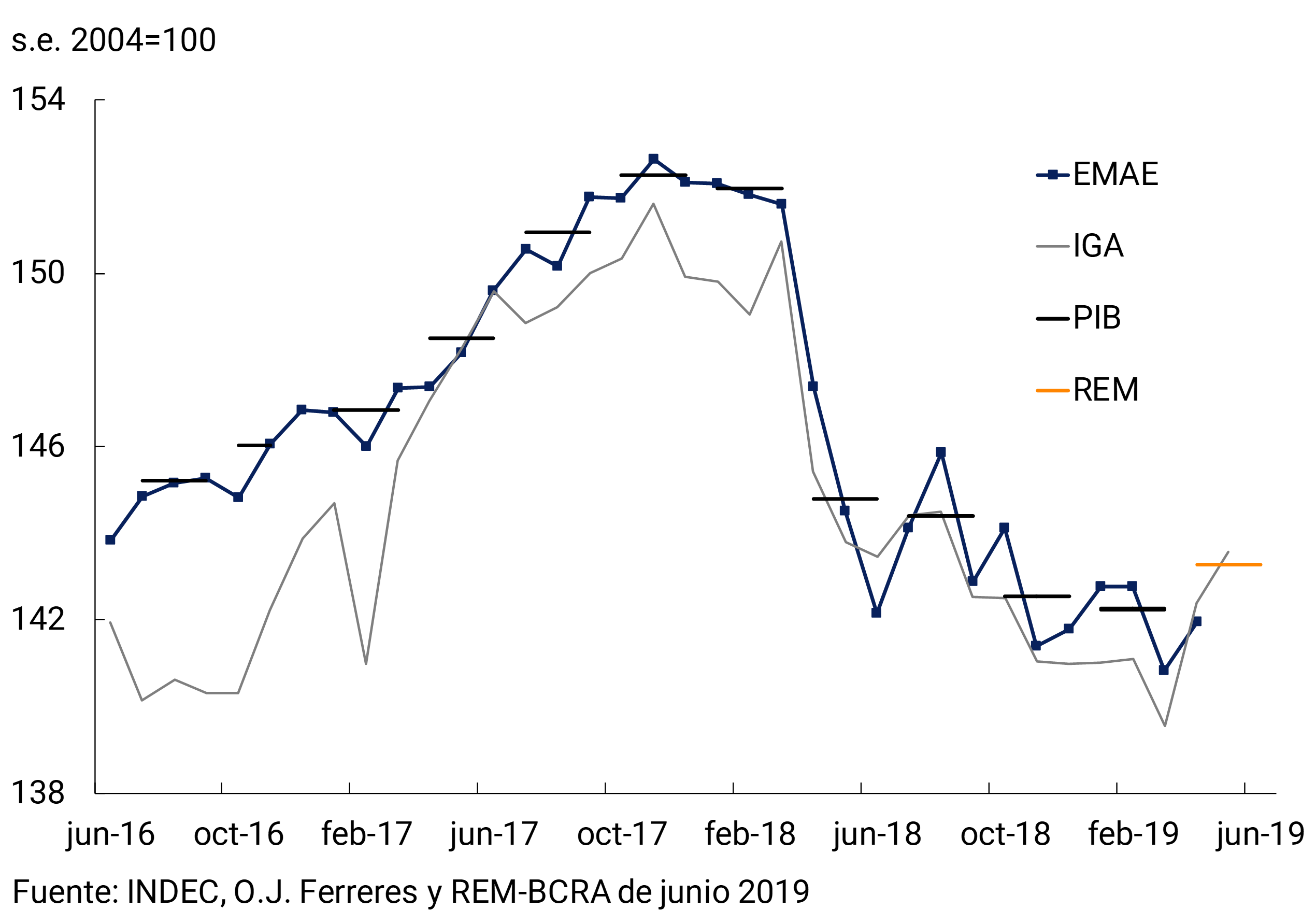
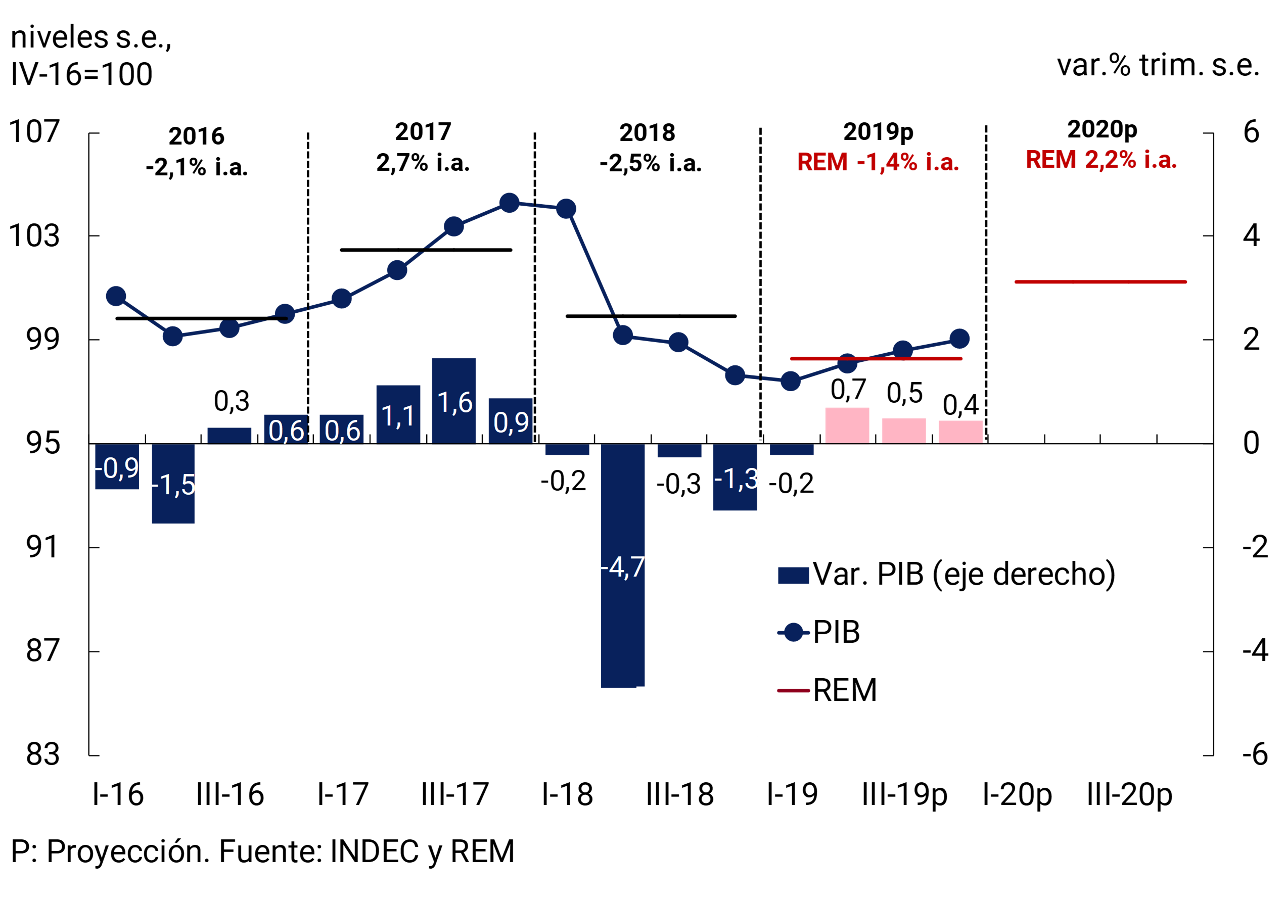
The Monthly Estimator of Economic Activity (EMAE) showed a recovery in April (0.8% s.e.), cutting the year-on-year contraction to 1.3% and leaving a statistical drag close to zero for the second quarter. The first available indicators for May and June allow us to affirm that activity would have grown during the second quarter. In the same vein, the median of the REM estimates for June stood at 0.7% seasonally adjusted quarterly growth. Although the latest Contemporary GDP Prediction (PCP-BCRA) still shows a fall of 0.56% quarter-on-quarter s.e. (see Figure 3.1), the incorporation of new data is expected to change the sign of the projection.
Figure 3.1 | Economic activity
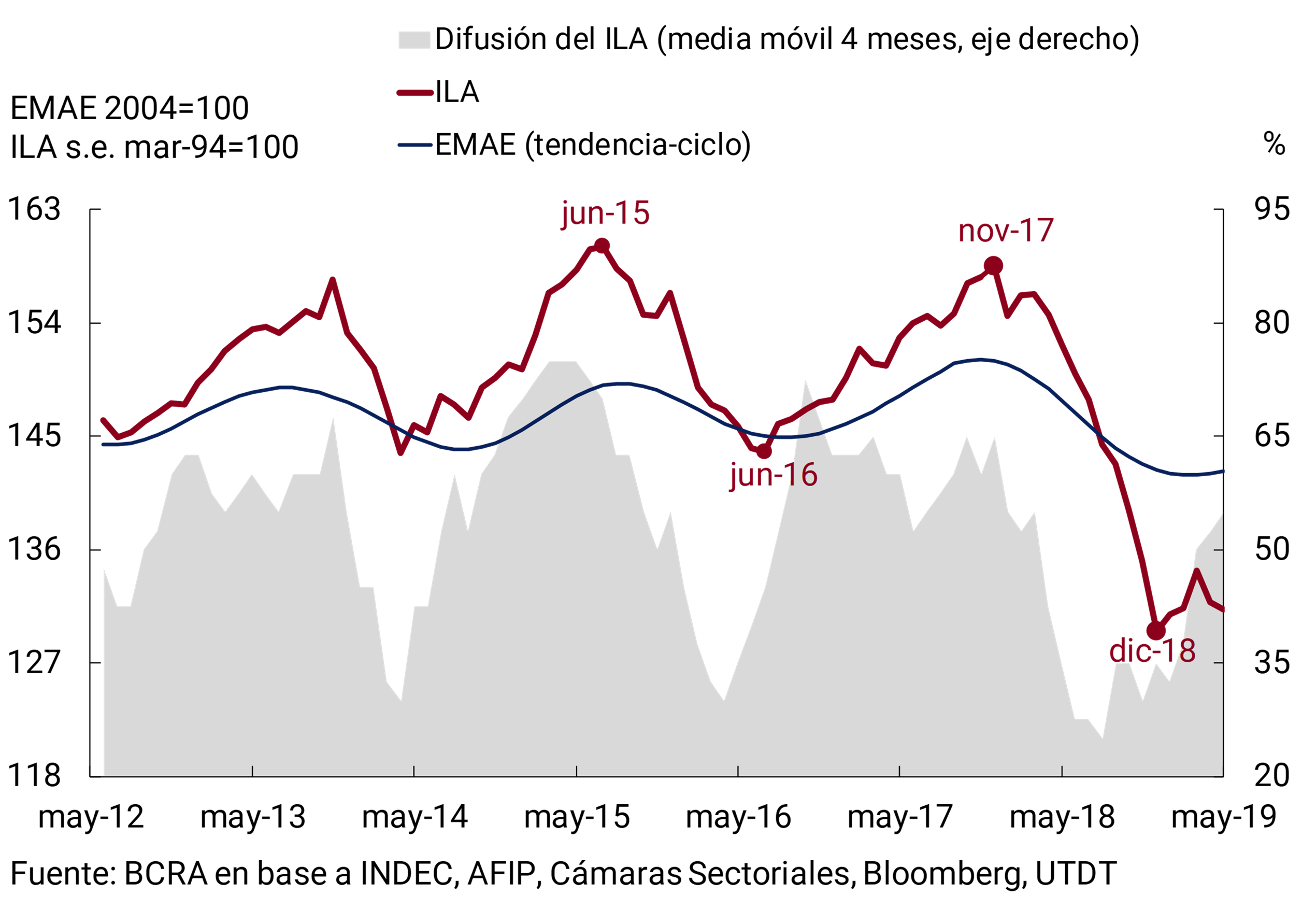
According to the Leading Activity Indicator (ILA), in May all the necessary criteria were met to confirm that the activity had entered an expansionary phase. Diffusion and depth exceeded the thresholds required to ensure the existence of a pivot point in the ILA in November 2018. In this way, the ILA anticipated the EMAE valley, which would probably be in March 2019 (see Figure 3.2).
Figure 3.2 | BCRA’s Leading Activity Indicator (ILA)
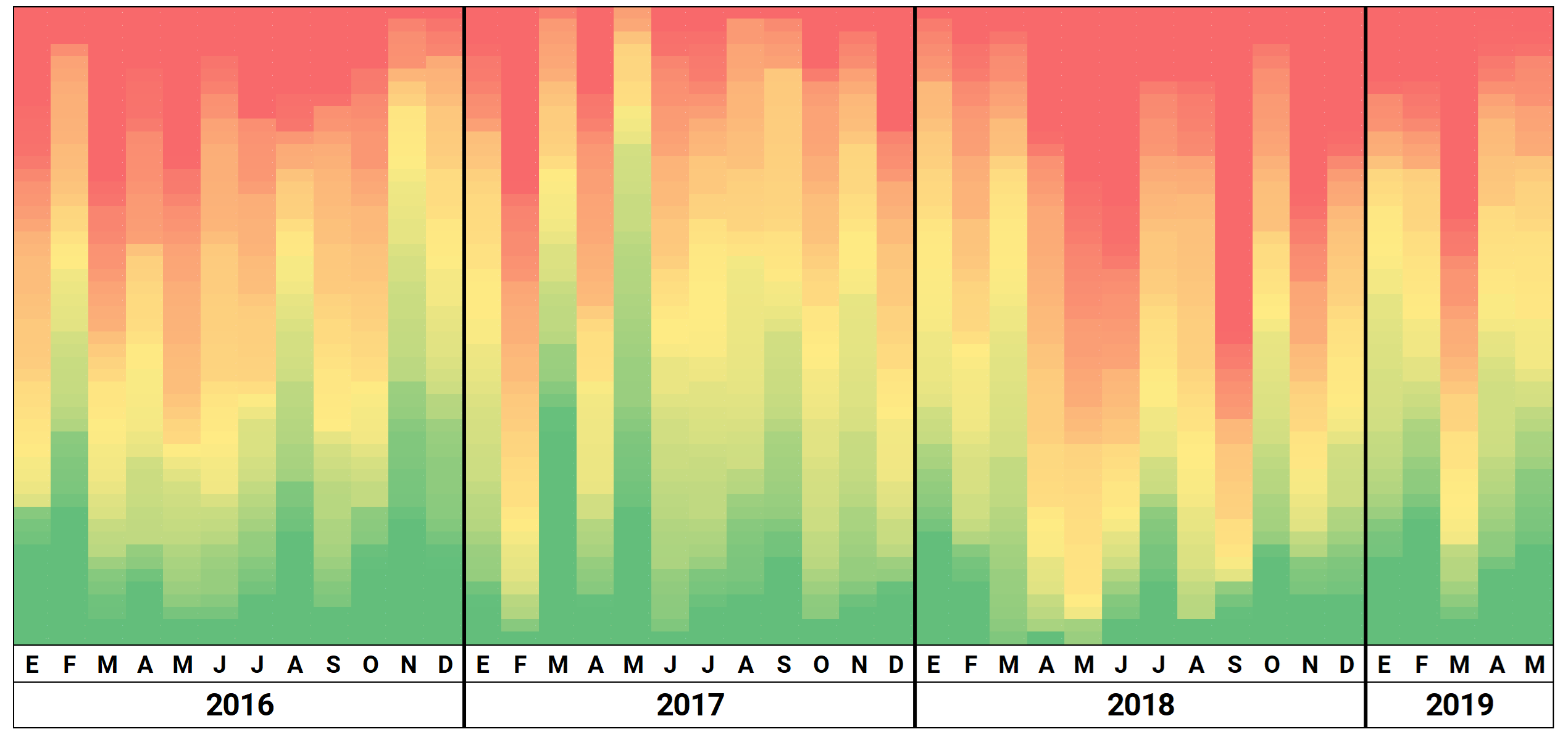
The diffusion and intensity of the growth of a broad set of activity indicators provides evidence in the same sense as the ILA-BCRA 6. As can be seen in the following graph, since December – with the exception of March – the growth of this group of variables has been more widespread and intense (the red areas have been reduced and the green areas have intensified; see Figure 3.3.).
Figure 3.3 | Intensity and sectoral diffusion of activity growth
Box: Corrections in seasonally adjusted series
The incorporation of new data to the original series modifies the series without seasonality as a result of the characteristics of the methods used to discard the seasonal component. These corrections are usually more important at the turning points of the series, affecting even the sign of the variation of the series without seasonality. This phenomenon was present in the EMAE series during the third quarter of 2016 and the first quarter of 2018, which are the last two turning points recorded so far (see Figure 3.4). The first EMAE publications for the third quarter of 2016 indicated that the economy continued to go through a recessionary phase. With the incorporation of new data, the variation of the EMAE without seasonality went from a fall of 0.9% to a rise of 0.3% in that period. In contrast, during the first quarter of 2018, the variation of the EMAE without seasonality went from an increase of 1.1% (first publication) to a fall of 0.2% (last publication).
Figure 3.4 | EMAE Monthly Corrections

Various consumption and activity indicators analyzed in this IPOM have been showing a recovery since December 2018. It is expected that the EMAE’s non-seasonality series for the first quarter of 2019 may be revised upwards with the incorporation of new observations to the original series.
3.1.1 Domestic demand began to recover
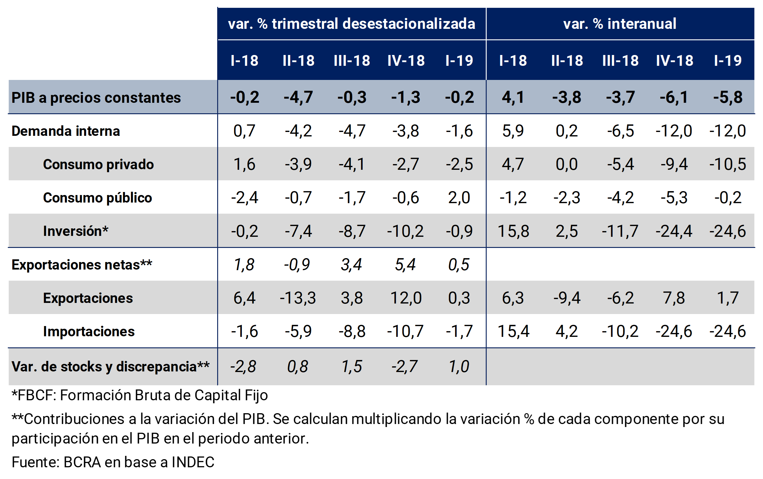
During the first quarter of 2019, domestic demand continued to deteriorate, although it slowed its decline (-1.6% quarter-on-quarter) due to the rise in public consumption (2.0% s.e.) and the sharp cut in the contraction of investment7 (-0.9% s.e.). Private consumption had another significant drop (-2.5% s.e.).
Net exports made a slightly positive contribution to the seasonally adjusted quarterly variation of GDP in the first quarter (0.5 percentage points (p.p.), as a result of the reduction in imports (-1.7% s.e.) – explained by the performance of domestic demand – and a slight increase in exports (0.3% s.e.). Finally, the change in stocks and the discrepancy had a positive contribution to the seasonally adjusted quarterly variation of GDP (1 p.p.; see Table 3.1).
Table 3.1 | Quarterly changes in GDP and contributions of its components
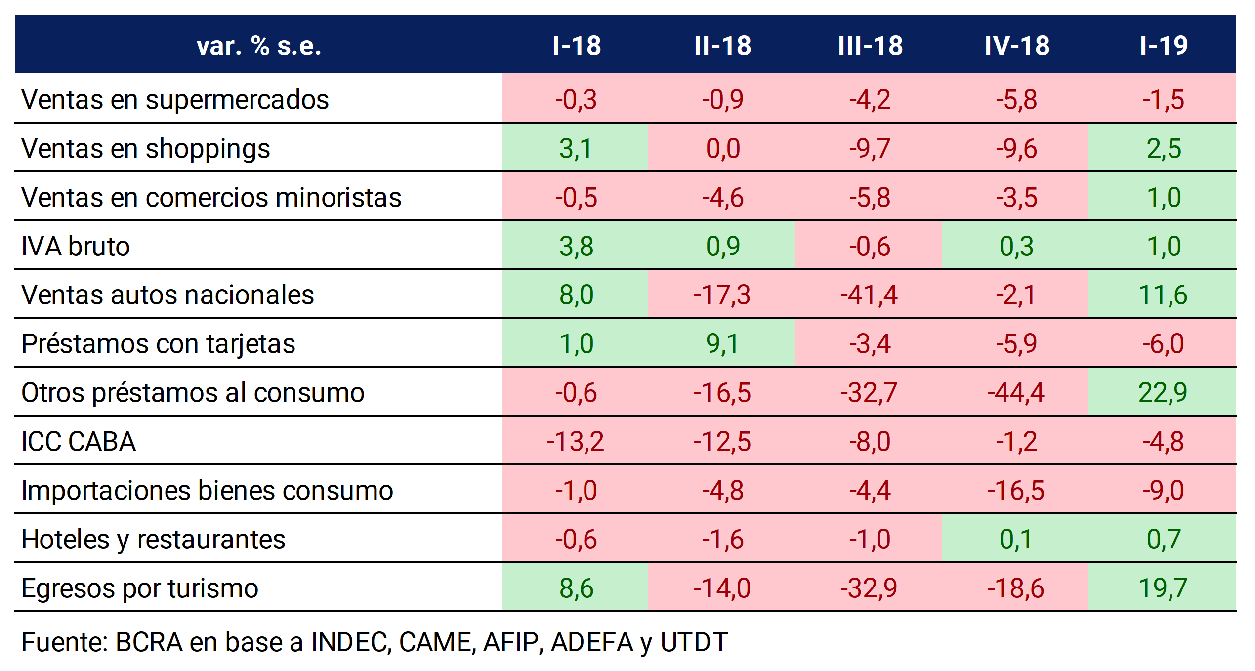
Private consumption registered a new fall during the first quarter of 2019 despite the fact that several partial indicators showed an improvement. Among them, the growth in sales volumes in shopping malls (2.5% s.e.), sales of domestic cars (11.6% s.e.) and the net granting of consumer loans (22.6%) (see Table 3.2) stand out.
Table 3.2 | Partial indicators of private consumption
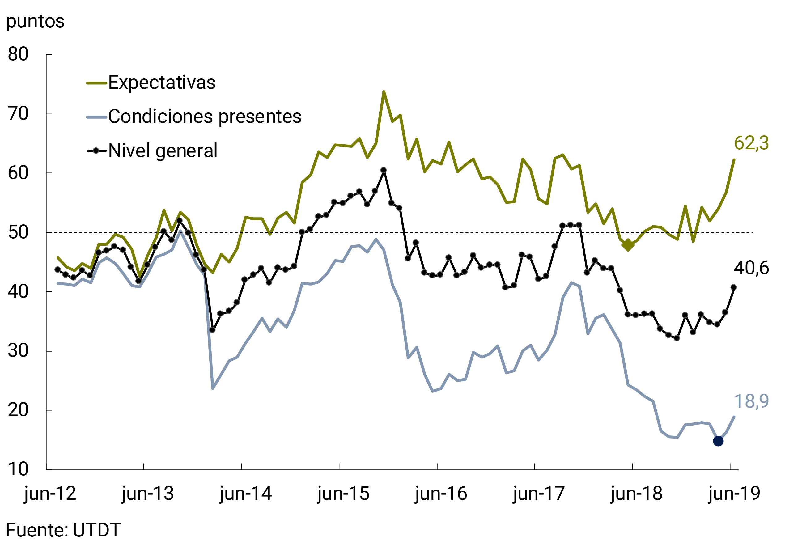
The BCRA’s Leading Indicator of consumption rose in the first quarter. This indicator usually anticipates the turning points of INDEC’s private consumption, so it allows us to expect a recovery in the second quarter (see Figure 3.5). For the remainder of the year, the expected recovery in income, together with the measures announced by the government (see box Measures to promote consumption), foresee good prospects for consumption. Some data related to household consumption in the second quarter showed a better performance. The Consumer Confidence Index of the Di Tella University at the national level (ICC-UTDT) rose 5.8 p.p. between March and June (2.5 p.p. quarterly on average), gross VAT collection (DGI + DGA) increased 4.5% s.e.8 and the quantities imported of consumer goods during the April-May two-month period increased on average 0.8% s.e. compared to the first quarter.
Figure 3.5 | Private Consumption and BCRA Leading Indicator

The expected recovery in revenues together with the measures announced by the national government (see Box: Measures to promote consumption) will boost consumption during the remainder of the year.
Box: Measures to promote consumption
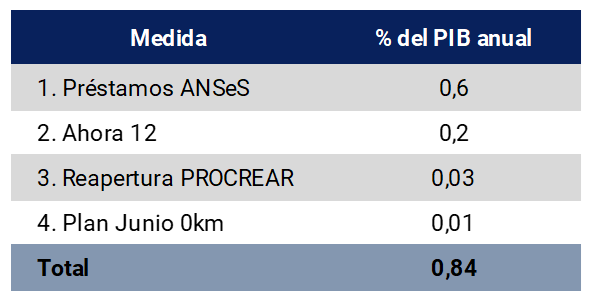
During the second quarter of 2019, the National Government carried out different measures to promote private consumption for an approximate amount of 0.8% of GDP. The full impact of these measures will be recorded between the third and fourth quarters of 2019.
The plans have different purposes such as the purchase of homes (PROCREAR), cars (June 0KM), household appliances (Ahora12) and personal expenses (ANSES) the main objective of these programs is to improve household consumption.
The line of credit granted by ANSeS9 is a program of personal loans for retirees, pensioners and those who receive Child Allowances. The amounts range from $5,000 to $200,000 in the first two cases, while those designated for AUH beneficiaries are in a range of $1,000 to $12,000. ANSES estimates that it will grant loans for $124,000 million until the end of the year, that is, 0.6% of GDP.
With the aim of “promoting consumption and national production of goods and services,” the quota purchase programs called Ahora 3, Ahora 6, Ahora 12 and Ahora 18 were launched. The rates for all cards issued by banks are 20%, which represents a decrease of 25 percentage points compared to the previous rate of the program (45%) effective from June 1 to December 3110. The financing granted could reach 0.2% of GDP in the second half of the year.
The launch of a new phase of the Procrear Plan allows access to credit for the purchase of housing, new or used, for family use and permanent occupation11. This line of credit is key in segments of the population that have housing needs or significant improvements in their homes.
To encourage car sales, the June 0km12 plan has bonuses that are around $50,000 and $90,000, according to the price of the chosen car. In addition, the City of Buenos Aires and the Province of Buenos Aires will reduce the stamp tax (to units of less than $750,000) that is charged with the patenting13. The fiscal cost of this program would be partially offset by the tax revenue derived from the sale of a greater number of cars. The different measures mentioned could together reach around 0.8 p.p. of GDP (see Table 3.3).
Table 3.3 | Estimation of the maximum amounts involved in the different programs as a percentage of GDP in 2019
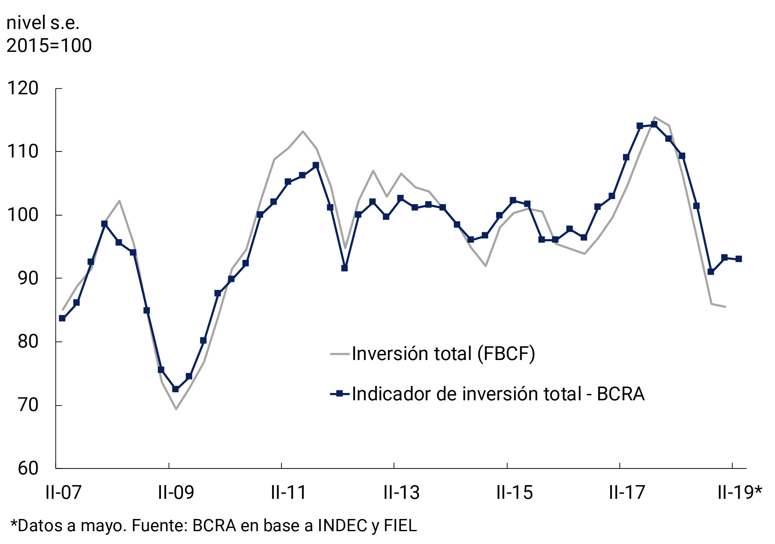
With respect to investment, the fall observed in the last quarter of 2018 (-10.2% s.e.) was considerably reduced. The contraction of 0.9% s.e. in the first quarter was explained by a sharp decrease in expenditure on Durable Production Equipment (-5.8% s.e.), which was attenuated by an increase in Construction (3.6% s.e.). With partial data from the second quarter, the BCRA-investment indicator—which had recovered slightly in the first quarter—remained stable (see Figure 3.6).
Figure 3.6 | Gross Fixed Capital Formation (GFCF) – Investment
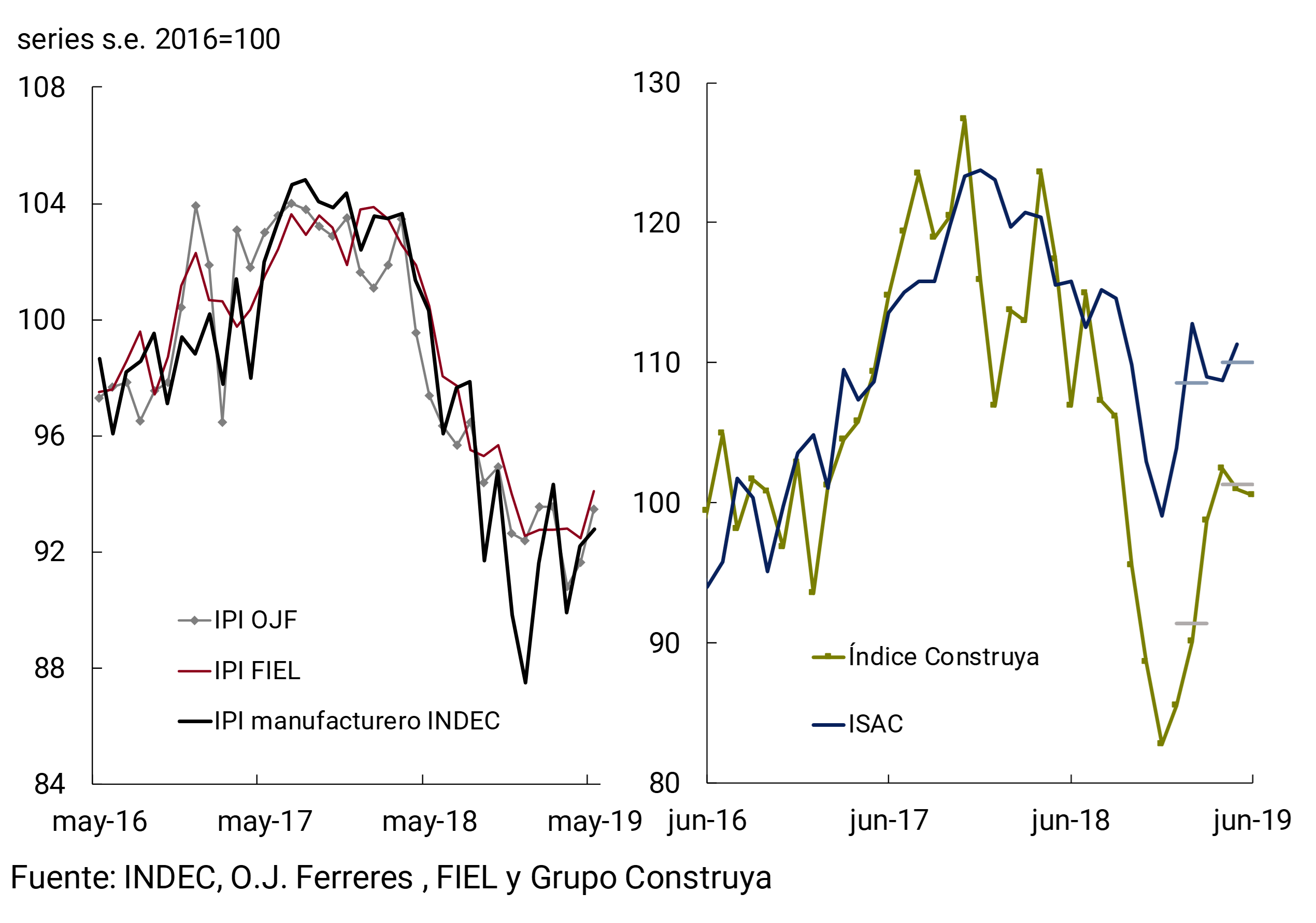
The Construction component of the Gross Fixed Capital Formation (GFCF) of INDEC would show a new increase during the second quarter of 2019. The Construya Index, which measures sales of the main construction inputs, increased 9.4% between April and May compared to the first quarter of 2019, while the Construction sector of the EMAE – an indicator that weights the demand for the main construction materials and the labor involved – 14 grew 0.8% s.e. in April compared to the first quarter of 2019 (see Chart 3.7).
Figure 3.7 | Construction Indicators
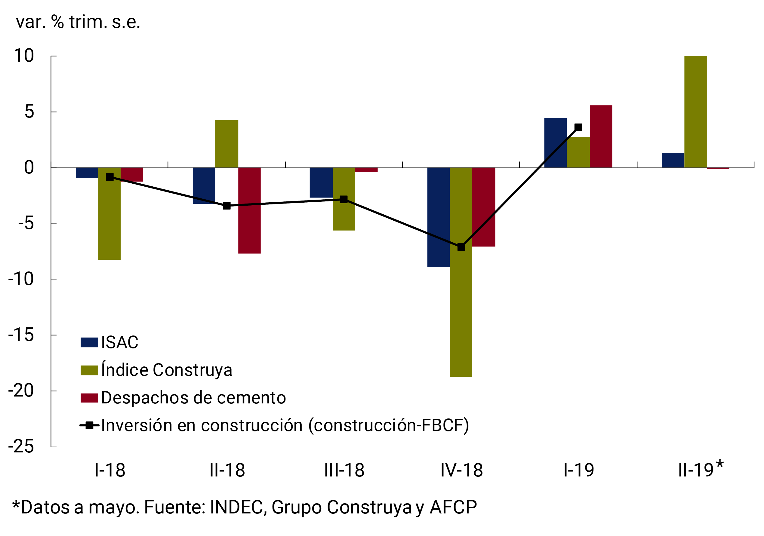
The good performance of construction was explained both by the reactivation of private works and by the faster pace of execution of public works. The greater dynamism of private works can be seen from the evolution of the inputs typically used in this type of construction, such as ceramic floors and coatings (+9.5% s.e. between April and May compared to the first quarter) and gypsum (+5.3% s.e. in the same period). As for public works, according to data from Construar15, the amounts involved in the calls for public tenders (from the national, provincial and municipal states) rose 61% y.o.y. in nominal terms in the first quarter of 2019, a figure that, deflated by the INDEC Construction Cost Index, meant an increase of 11.1% y.o.y. in real terms.
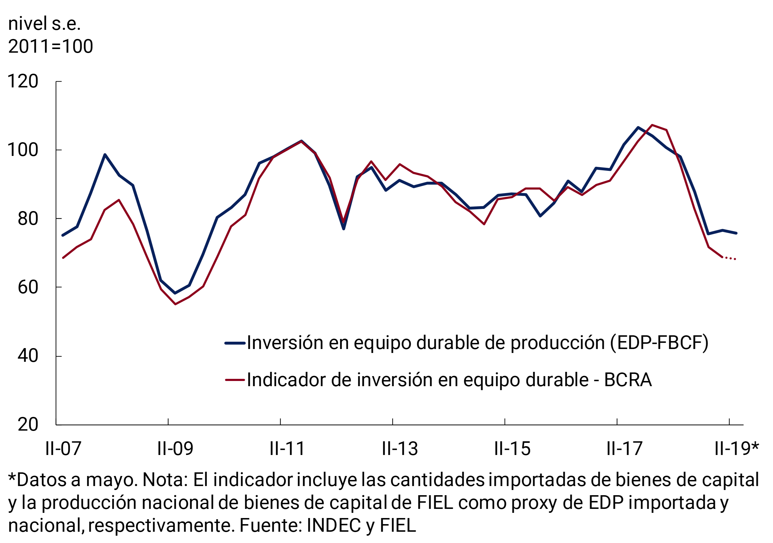
The BCRA’s Durable Equipment Investment Indicator remained stable during April and May compared to the previous quarter. The improvement in demand for imported equipment was offset by the fall in domestic production of capital goods surveyed by FIEL, which has a high correlation with investment in domestic equipment (see Figure 3.8).
Figure 3.8 | Investment indicators in durable production equipment
3.1.2 In the second quarter, exports of goods were driven by the agricultural sector
In the first quarter of 2019, real exports of goods and services showed slight growth (0.3% qoq s.e. and 1.7% y.o.y.), while imports fell again (-1.7% s.e. and -24.6% y.o.y.), partially offsetting the contraction in domestic demand. The slight improvement in total exports was explained by higher exports of services, particularly travel, which more than offset the decline in exports of goods in the quarter (see Figure 3.9).
Figure 3.9 | Foreign trade in goods and services
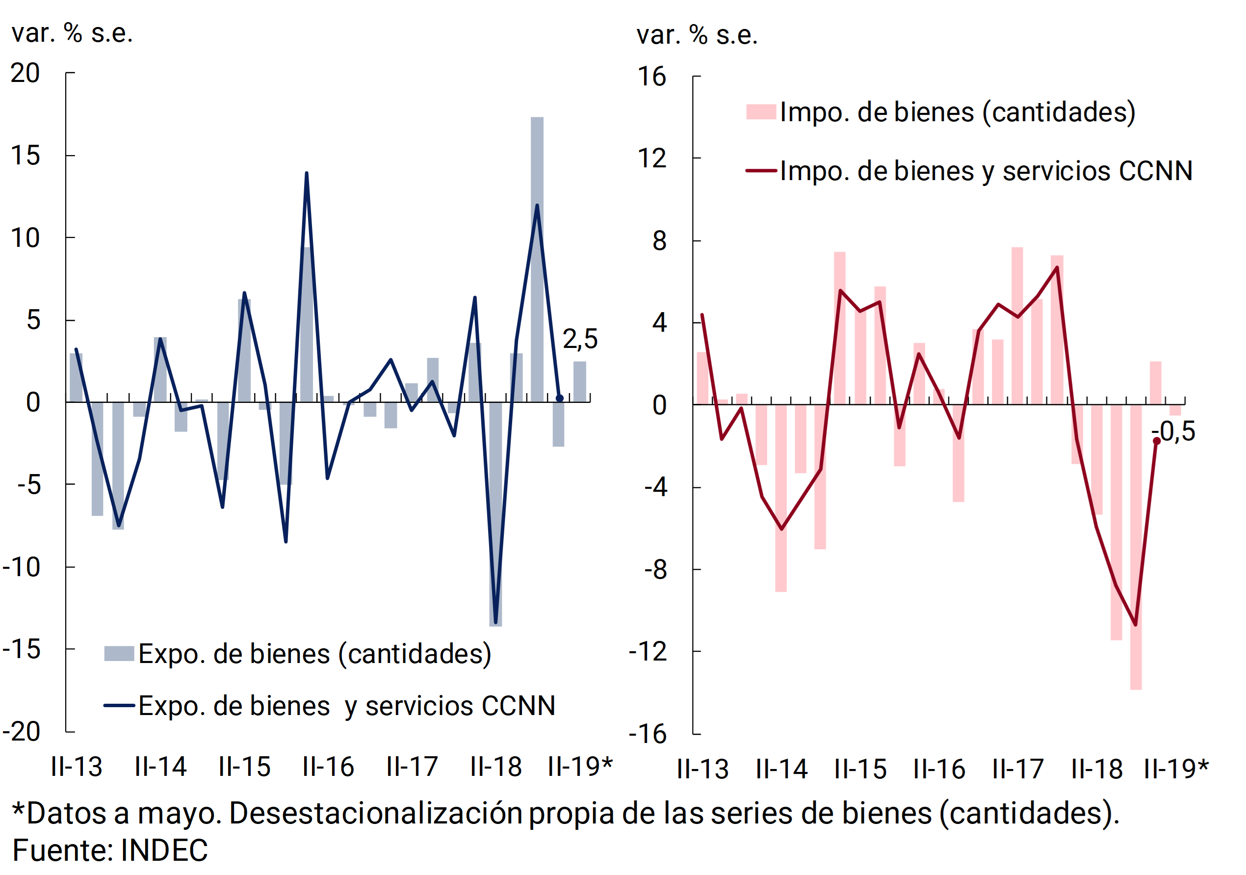
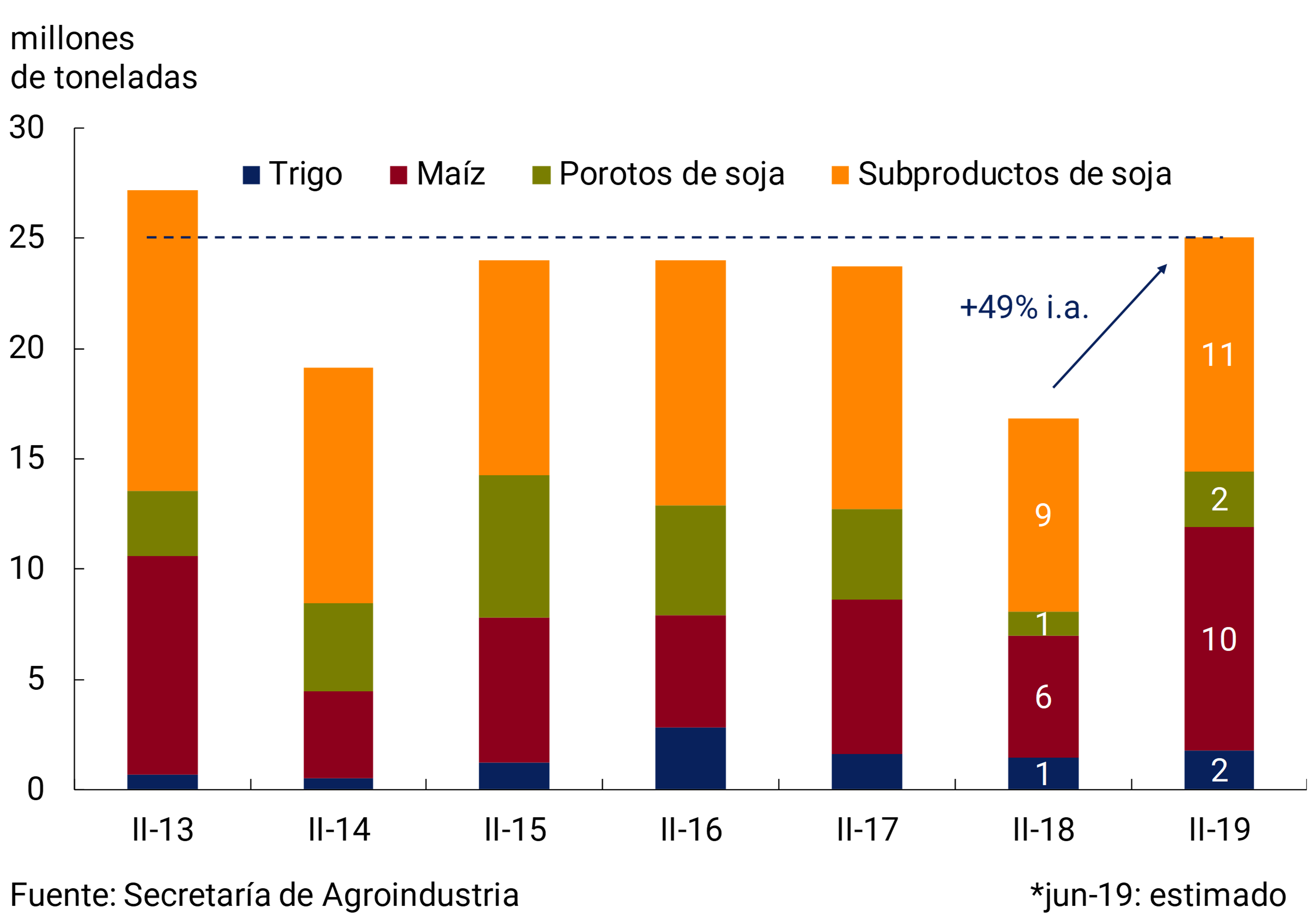
In the two months of April-May 2019, exports of goods rose 2.5% s.e. compared to the previous quarter. This performance was more influenced by shipments of cereals (22% s.e.) and soybean by-products (6% s.e.). Advance shipment data suggest that the good performance of products linked to the record harvest was sustained in June. The total shipped of the main grains and their derivatives increased 47% YoY in the second quarter, reaching the highest cumulative since II-13 (see Figure 3.10).
Figure 3.10 | Main grains and soybean derivatives. Tonnage shipped
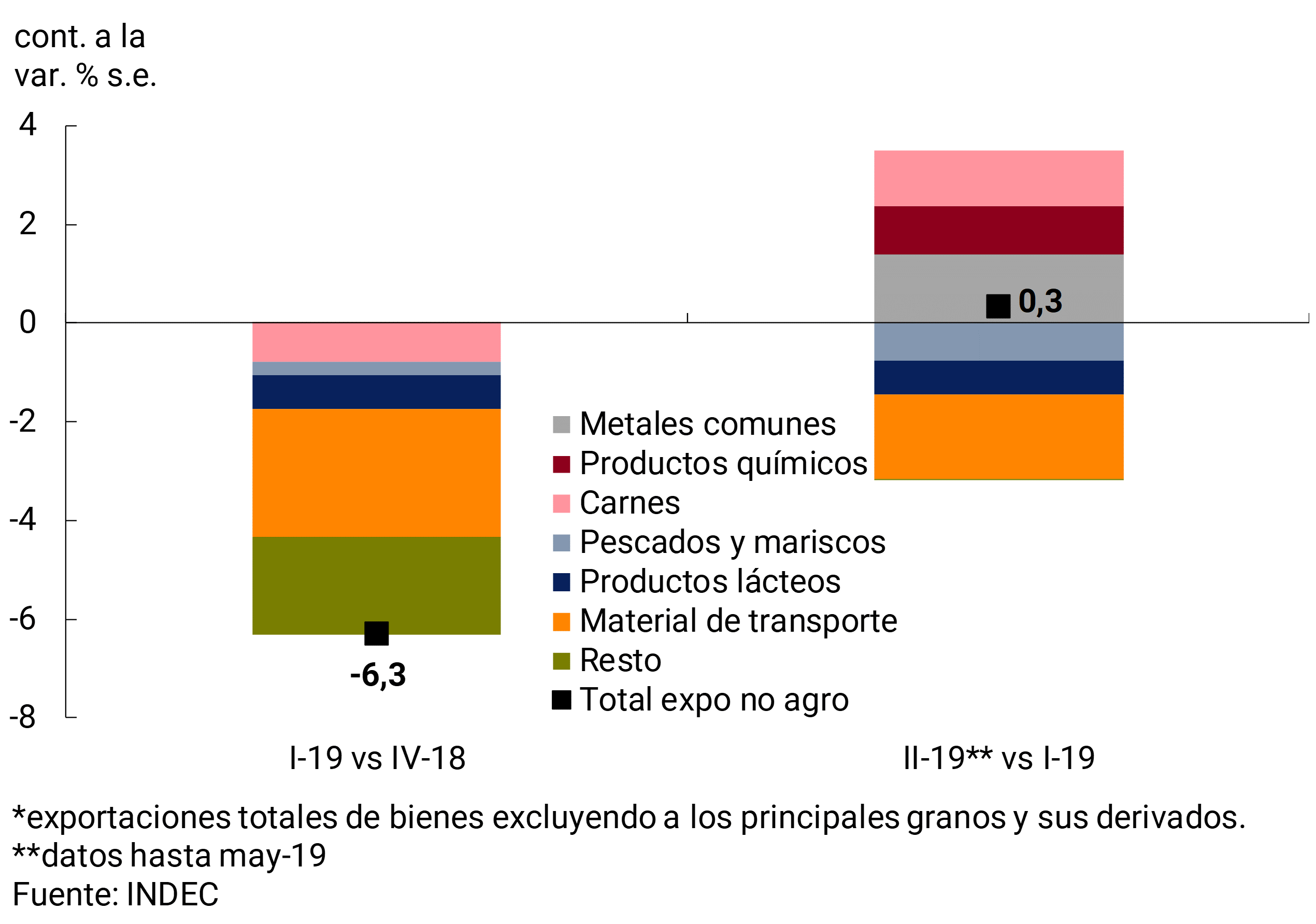
In the April-May period of this year, non-agricultural exports rose by just 0.3% s.e. after a negative first quarter in which they fell widely. In any case, they were 1.7% above last year and accumulate a seasonally adjusted increase of 27% compared to the minimum of Dec-15. The sectors that showed a recovery in exports during the second quarter compared to the previous quarter were: base metals (22% s.e.; 27% y.o.y.), meat (19% s.e.; 33% y.o.y.) and chemical products (10% s.e., 2% y.o.y.). On the other hand, external sales of land transport material, dairy products, and fish and seafood fell for the second consecutive quarter and were lower than those of the same period in 2018 (see Figure 3.11).
Figure 3.11 | Non-agricultural exports*. Quantities exported s.e.
On the other hand, in the April-May two-month period, imported quantities registered a slight drop (-0.5% s.e. compared to the first quarter), explained by the negative carry-over left by the March data (-6.5% s.e.). Both April and May saw monthly increases (5.3% s.e. and 2.1% s.e., respectively). At the disaggregated level, the purchases of parts and accessories for capital goods (12% s.e.) and chemical inputs (8% s.e.) stood out for their incidence. Despite this recent increase, in May the volumes acquired were 31% s.e. below the previous maximum reached in Nov-17.
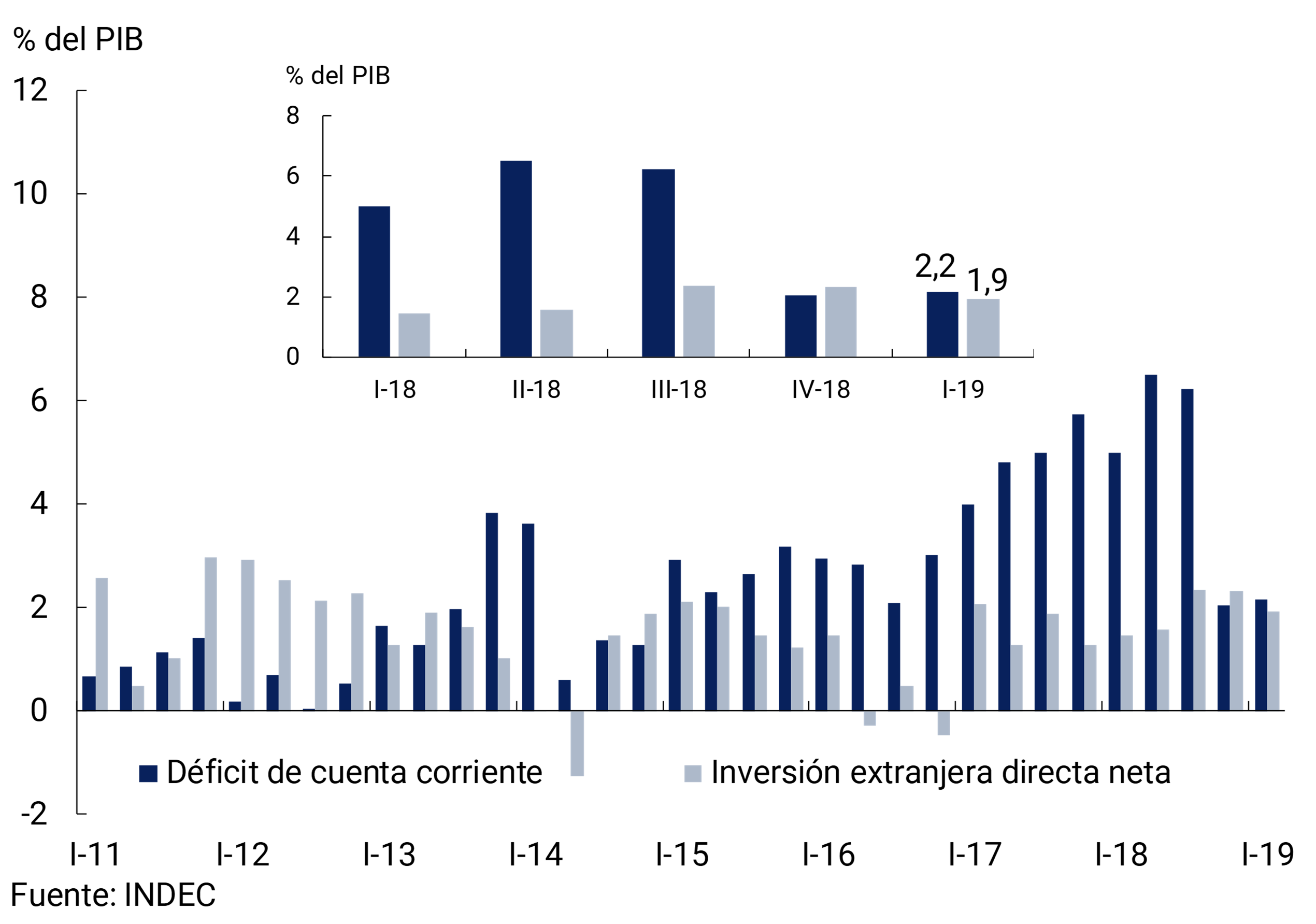
This evolution of trade flows of goods in the second quarter shows the continuity of the process of correction of the external accounts of the Argentine economy that began in the second half of 2018. The rise in the real exchange rate during 2018 allowed the Argentine economy to start the year with a seasonally adjusted and annualized current account deficit of around 2% for the first time since 2014, a level similar to the annual net income from foreign direct investment that Argentina receives (see Figure 3.12).
Figure 3.12 | Current account and foreign direct investment (annualized securities)
For the remainder of the year, exports are expected to continue to be driven mainly by the agricultural sector. After a record harvest, 73% of soybean exports, 60% of by-product sales and 44% of corn shipments estimated for 2019 would be completed in the second half of the year (see Agricultural Harvest). For its part, it is estimated that, after having found a floor in March, imports will consolidate a reactivation, to the extent that economic activity demands it.
3.1.3 Major sectors of the economy continue to recover
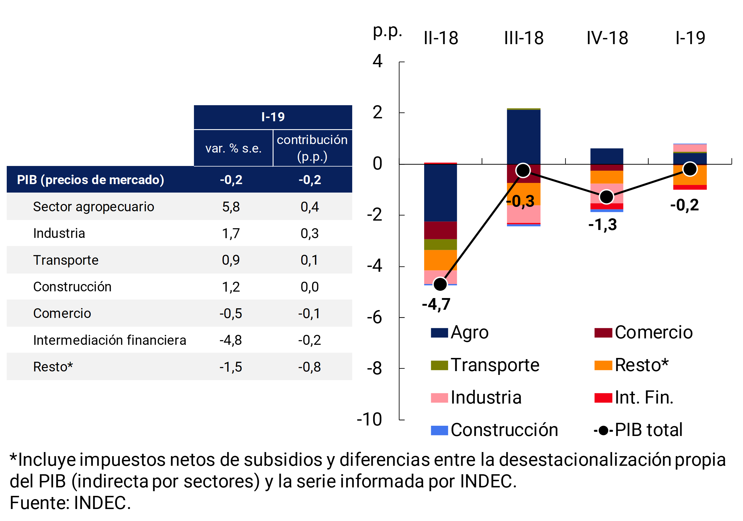
The slight fall in the economy during the first quarter (-0.2% s.e.) was explained by the transitory fall in activity in March and was concentrated in only four of the sixteen sectors of GDP. A number of important activities – Agriculture, Industry, Construction, Mining and Quarrying, and Transport – grew compared to the previous quarter.
The contractions with the greatest incidences were registered in Financial Intermediation and Commerce, affected by the reduction in private consumption and exchange rate instability in March. Electricity, Gas and Water, Other Community Service Activities and the tax component net of subsidies accounted for the rest of the fall in GDP measured at market prices (see Figure 3.13).
Figure 3.13 | I-19 Sectoral Economic Activity
The level of activity improved again in April, reaching above the level of December 2018 in eleven of the fifteen sectors that make up the EMAE. According to different available indicators, relevant sectors such as industry and construction would have grown during the second quarter compared to the first quarter (see Figure 3.14).
Figure 3.14 | Industry and Construction recover
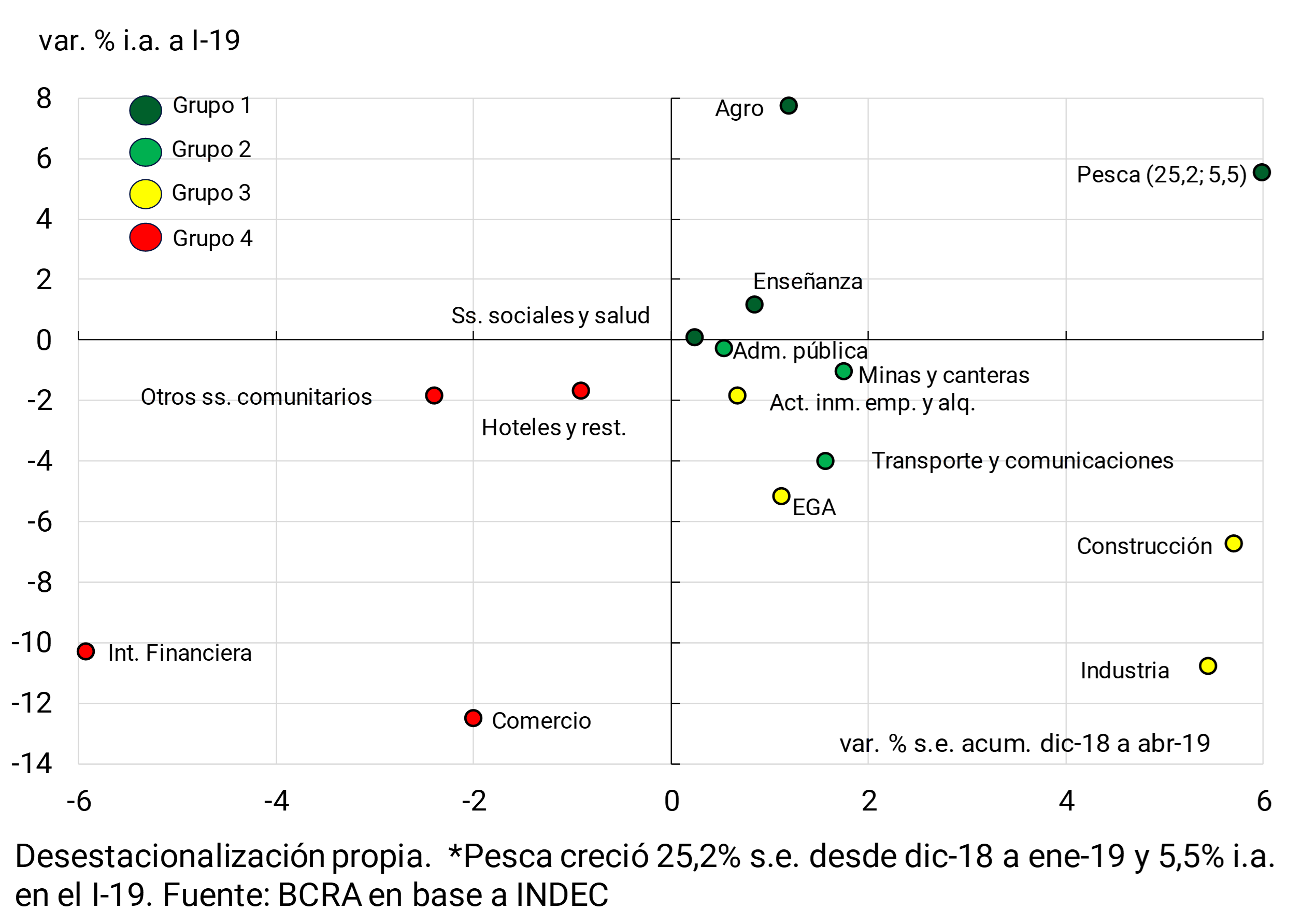
The performance of economic activity since the end of 2018 has not been homogeneous among the different productive sectors. In line with the classification made in the last IPOM of April 2019, the sectors can be separated into four groups according to their recent evolution.
Group 1 – Agriculture, Fisheries, Education and Social and Health Services – is made up of the activities that have been improving since mid-2018 and that during the first quarter of 2019 reached or exceeded the level of the same period of the previous year. The most relevant sector of this group is Agriculture, which rebounded in the third quarter of 2018 (in seasonally adjusted terms) after the fall caused by the drought, and since then it has continued to grow thanks to the good harvest of the main crops (see Agricultural Harvest Section). According to EMAE data, agricultural produce grew 40.2% year-on-year in April. On the other hand, the Fisheries product was not affected by the recession and performed well in 2018 (5.4% YoY). The growth continued during the first months of 2019, registering a year-on-year increase of 35% in April. Meanwhile, Education and Health services slowed down during 2018 without entering a recessionary phase16.
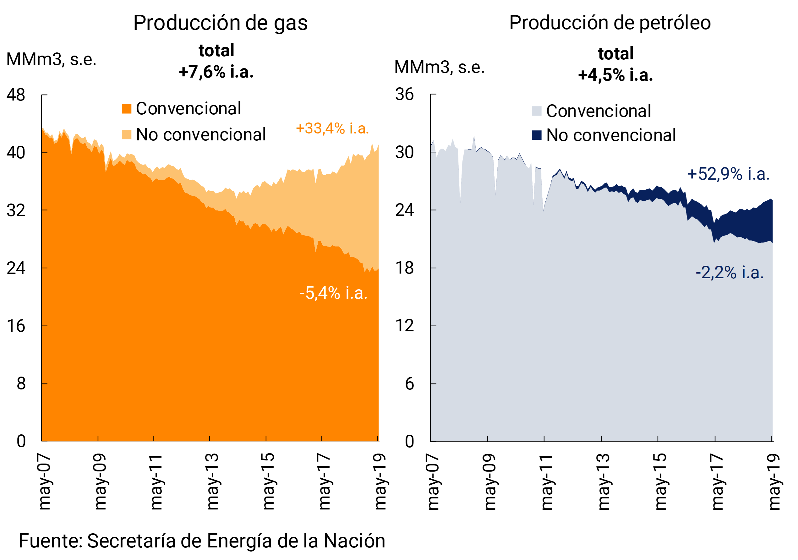
Group 2 – Mining and quarrying, Public Administration and Transport – is made up of sectors that recovered since the end of last year and that, if the recent trend continues, could grow in year-on-year terms during the second quarter of 2019. Oil (+4.5% YoY in May) and Gas (+7.6% YoY in May) production leads the Mining and Quarrying sector with a multiplier effect on other economic sectors. The extraction of unconventional oil and gas from the Vaca Muerta field grew by 52.9% YoY and 33.4% YoY, respectively, outpacing the decline in production from conventional wells (see Figure 3.15). The Transport sector has been recovering, driven by the growth of agriculture and tourism, and is expected to reach a positive year-on-year growth rate of between 1% and 2% in May. Within the framework of a process of fiscal consolidation, the public administration sector has registered a structural breakdown since 2016, growing at a low rate in historical terms17. Between December 2017 and August 2018 it accumulated a contraction of 1% and then began to recover, reaching a slight growth of 0.2% y.o.y. in April.
Figure 3.15 | Unconventional hydrocarbons drive the energy sector
Group 3 includes sectors that have begun to reactivate since the end of 2018 but, due to the depth of the previous decline, it will take longer for them to reach pre-recession levels. This group – Industry, Construction, Real Estate Activities and Production of Electricity, Gas and Water – is the one with the greatest weight in the economy (35%). The EMAE of April 2019 and the data available as of June18 indicate that this group of activities would have grown in the second quarter of the year compared to the first. The improvement was mainly explained by the recovery of domestic demand, in a context of greater exchange rate stability, which was added to the aforementioned indirect impulses from agriculture and the hydrocarbon production sector.
Group 4 – Trade, Financial Intermediation, Hotels and Restaurants, and Other Community Services – is made up of the activities of the EMAE that have not yet managed to reverse the declining trajectory. Trade, which had begun to recover in December 2018, fell sharply in March and, unlike the rest of the main sectors, did not recover in April. Financial intermediation continued to be affected by the tightening of financial conditions that increased the cost and reduced the demand for bank loans. The favorable boost from higher inbound tourism in the Hotels and Restaurants sector has so far not been able to offset the contraction in domestic demand, resulting in a level of activity for April 2019 similar to that of the third quarter of 2018. This group of sectors is expected to begin a recovery as the improvement in the rest of the economic activities is consolidated during the coming quarters of 2019 (see Figure 3.16).
Figure 3.16 | Recent performance of sectoral economic activity
3.1.4 Registered employment was sustained so far this year
Total registered employment maintained its level in the first four months of the year after 11 months of downward trend, in line with signs of improving economic activity. After a slight rebound at the beginning of the year, interrupted in March by exchange rate instability, it returned to marginal growth in April (see Figure 3.17).
Figure 3.17 | Total registered employment (e.g.; excluding the social monotax)
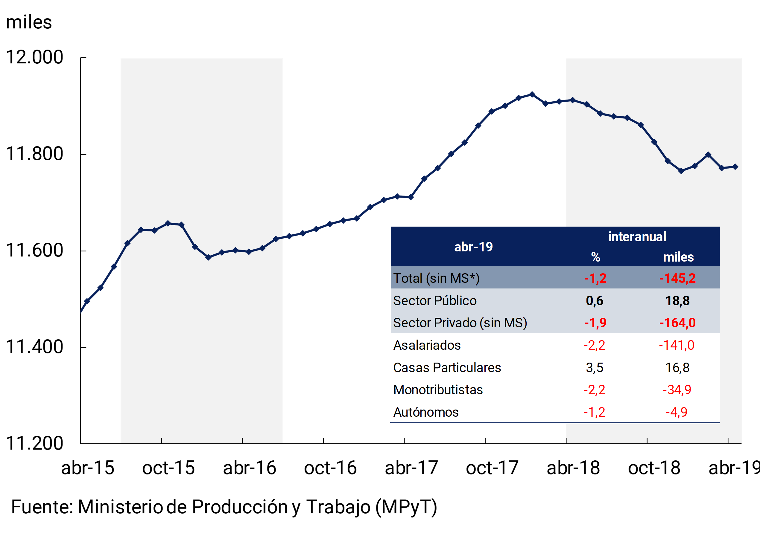
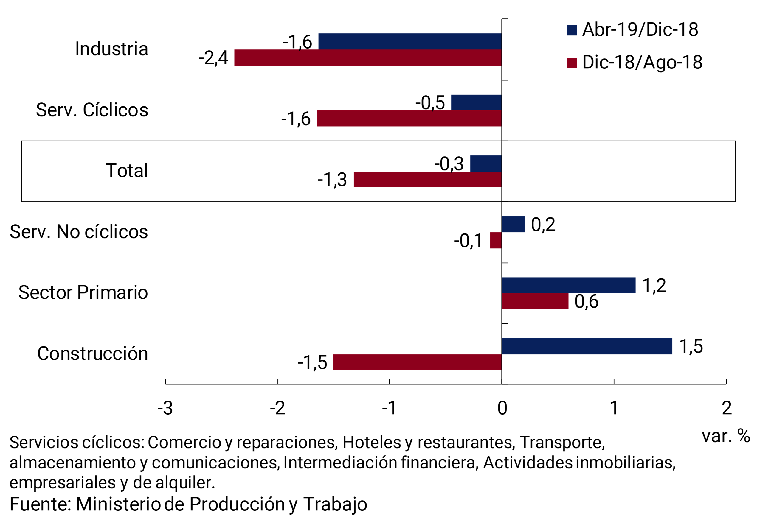
During the first four months, registered employment was sustained by the increase in public salaried employment (0.7% s.e.) and private households (1.2% s.e.), while self-employed and private salaried employment exhibited falls (-0.1 s.e. and -0.3% s.e., respectively). Private salaried employment attenuated its fall during the period due to the good performance of the primary sector and the recovery of construction, in a context in which jobs in industry and cyclical services continued to fall. (see Figure 3.18).
Figure 3.18 | Salaried employment registered by sector (not seasonal)
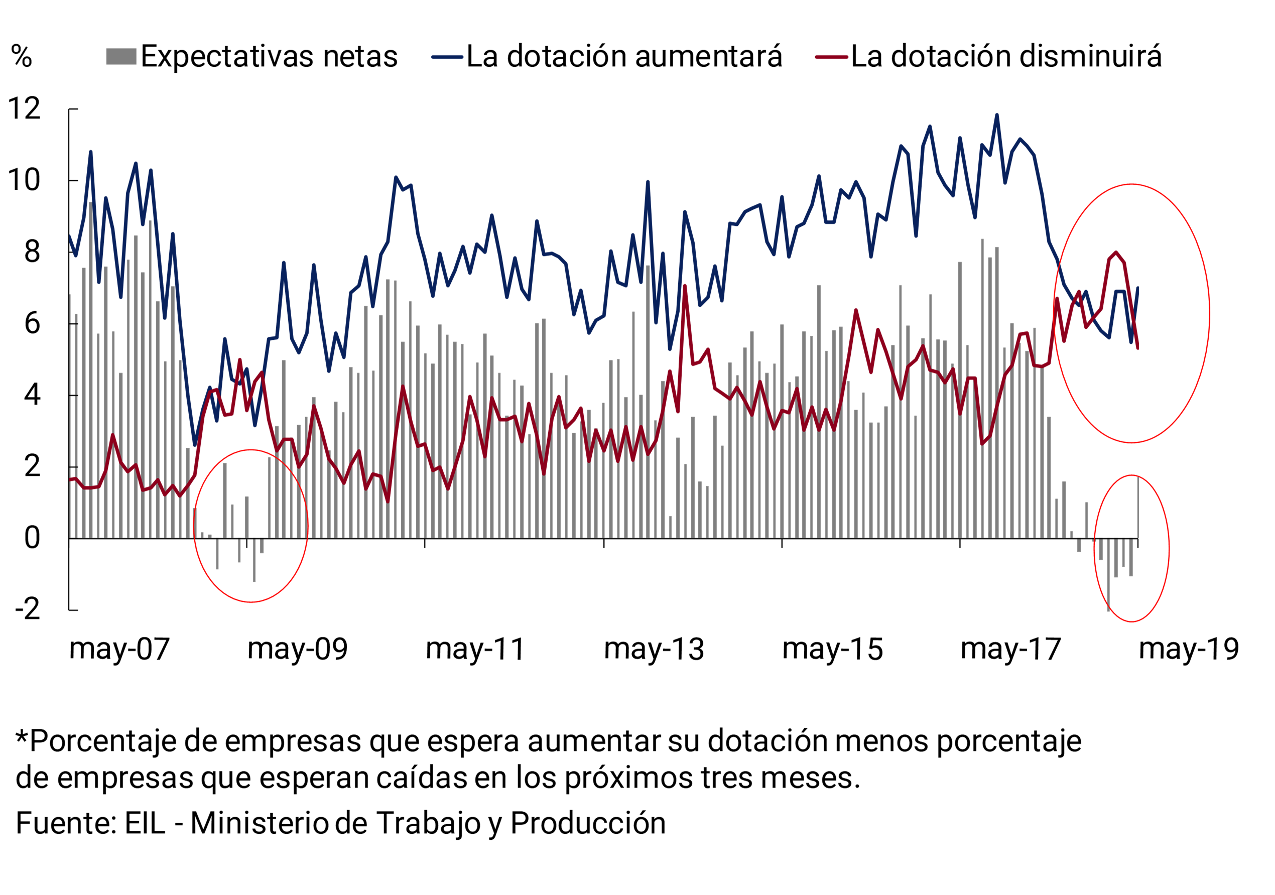
Companies expect a recovery in formal employment starting in June. According to the May survey of the Labor Indicators Survey (EIL), job creation expectations for the next 3 months were positive, after 6 months with negative records. This result was mainly due to a significant drop in staff reduction expectations and an expected increase in staffing (see Figure 3.19).
Figure 3.19 | Employment expectations
According to EPH figures, during the first quarter the informal sector and self-employment continued to offset the impact of the fall in registered employment. This made it possible for the employment rate to exhibit relative stability in the last year19. This growth in employment failed to cover that of the labor supply, leading the unemployment rate to reach 10.1% y.o.y. (1 p.p. year-on-year).
This change in composition in favor of jobs with lower labor intensity and/or lower remuneration, intensified pressures on the labor market. As usually happens in recessions, more people went out to look for work and/or more hours to complement their working day. As a result, in the first quarter the number of people with employment problems (work pressure) increased from 29.9% of the population to 33.9% (4.0 p.p. year-on-year; see Figure 3.20).
It is expected that the expected recovery of formal work from June, in a context of growth in economic activity, together with the improvement in family incomes will begin to reverse the pressure on the labor market.
Figure 3.20 | Economically active population and pressure on the labour market

3.2 Outlook
The favorable outlook in several sectors allows us to foresee a good performance of economic activity for the remainder of 2019. In addition to the direct and indirect impact of the record agricultural harvest and the continued development of gas and oil production from the Vaca Muerta field, there was a boost from activities producing tradable goods and services favored by a higher real exchange rate and greater market opening. This view is shared by REM analysts who project a stage of recovery and growth during 2019 and 2020 (see Figure 3.21).
Figure 3.21 | REM analyst projections
The record agricultural harvest, still in process, will continue to boost various economic activities directly or indirectly linked to production, such as the marketing and transport of agricultural products (see box Agricultural Campaign).
The energy sector will continue to show a good performance because its investment plans remained unchanged. The expected increase in oil and gas production in the coming years will reduce the external deficit20.
The domestic market will be strengthened by the expected improvement in household incomes in a context of falling inflation. Along the same lines, households find themselves with a debt-to-income ratio eased after several months of falling consumer loans with respect to output21. This will allow them to carry out a certain level of consumption previously postponed through the recovery of credit and the implementation of different consumption financing programs such as Ahora 12, Argenta, Junio/Julio 0Km (see box measures to promote consumption). Along these lines, the improvement in consumer confidence (ICC-DiTella) since January 2019 allows us to anticipate a recovery in the sale of durable goods and real estate for the current year (see Figure 3.22). Finally, investment in the construction sector will be driven by the fall in construction costs in relation to housing prices in a context of improved economic expectations.
Figure 3.22 | ICC-DiTella Expectations
Since December 2015 and within a framework of openness to international trade, new markets have been opened for Argentine products and pre-existing trade agreements have been deepened22. After a negotiation that lasted more than two decades, an agreement was signed with the EU with the aim of expanding and diversifying our exports, as well as stimulating investment and competitiveness through a better insertion of our economy in global production chains. Although the agreement is broad and the details of it are still under study, a high impact is expected in the coming years on FDI23, the export of agro-industrial goods24 and knowledge services25, a sector in which Argentina is beginning to stand out (see IPOM of April 2019).
Although the international context in which emerging economies operate has improved, some risk factors could condition this scenario of progressive recovery of activity (See Chapter 2. International Context). At the local level, the economic recovery scenario could be affected by some risks, mainly linked to a new episode of volatility in global financial conditions or to the usual uncertainty of electoral processes. In any case, in the context of the reduction of fiscal and external imbalances, a stronger balance sheet of the BCRA and a monetary regime in which the policy interest rate reacts immediately to developments, the space for local financial volatility events to occur is more limited (see Chapter 5. Monetary Policy).
4. Pricing
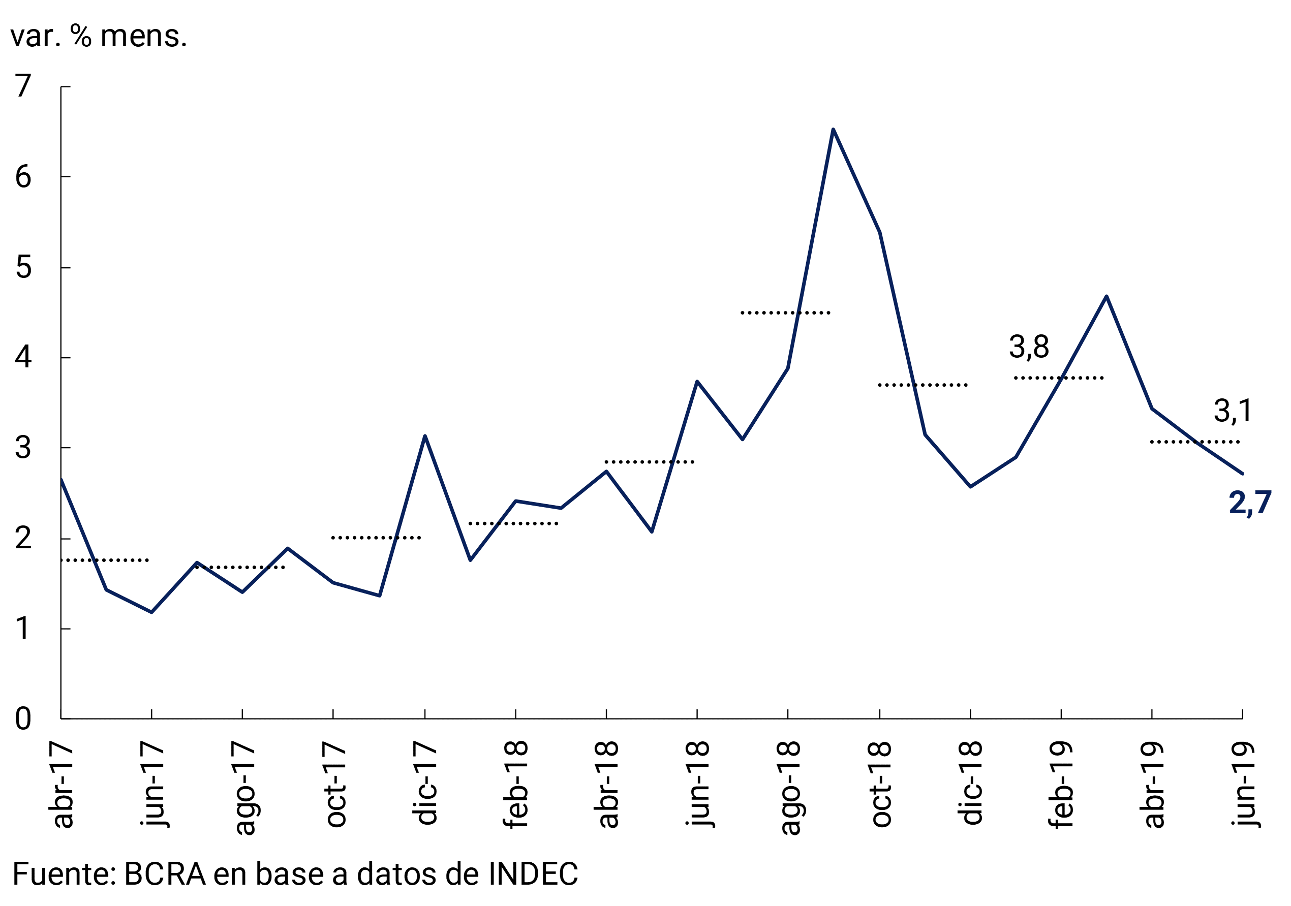
In the second quarter of the year, inflation showed some moderation, reversing the acceleration of the first quarter. This behavior in prices was generalized at the level of categories (Seasonal, Regulated and Core). In June, inflation stood at 2.7%, the lowest value of the year. However, it remained at high levels, with an annualized rate of around 38%.
The factors that had explained the acceleration of inflation during the previous quarter were attenuated in the second quarter. Corrections in utility rates continued, but to a lesser extent than in the first quarter of the year. Likewise, the supply shocks that had affected the price of meat were diluted. The tightening of monetary policy and the possibility of intervening within Exchange Reference Zone26 by the BCRA contributed to reducing exchange rate volatility and moderating inflation.
The contractionary bias of monetary policy, coupled with the fact that most of the correction in utility tariffs has already taken place, suggests that inflation would continue to fall in the coming months. This view is shared by market analysts who anticipate a downward path in inflation for the second half of the year. The Market Expectations Survey (REM) expects an average monthly increase in inflation of 2.3% for the period between July and December 2019 (30.8% annualized), reaching an inflation of 40% y.o.y. at the end of the year. Likewise, expectations indicate that the disinflation process would continue throughout next year, consistent with a more sustainable monetary policy framework.
4.1 In the second quarter, inflation figures were lower than those observed in the first months of the year
During the second quarter of the year, retail inflation moderated, reversing the upward trend of the first three months. The average monthly increase in the National CPI was 3.1%, 0.7 percentage points (p.p.) below the increases in the first months of 2019. The slowdown was generalized at the level of categories (Seasonal, Regulated and Core). In any case, inflation remains at high levels, reaching a monthly rate of 2.7% in June, equivalent to an annualized rate of around 38% (see Figure 4.1).
Figure 4.1 | National CPI. Monthly Evolution
The moderation in the inflation rate in the second quarter of the year was anticipated by the REM. The survey in March of this year predicted a rise in prices for the second quarter of 8.8%. In that period, the cumulative variation of the National CPI was 9.5%, only 0.7 p.p. above the data forecast by market analysts.
The factors that had driven inflation during the previous quarter were attenuated in recent months. After inflation hit 4.7% in March, it fell to an average of 2.7% in June, the lowest record so far this year. Lower inflation was basically due to the greater contractionary bias of monetary policy and the absence of new supply shocks. The tightening of monetary policy and the possibility of interventions within the exchange rate reference zone contributed to reducing the volatility of the exchange rate (see Chapter on Monetary Policy). The latter allowed to mitigate the upward pressures on the prices of the goods included in the index.
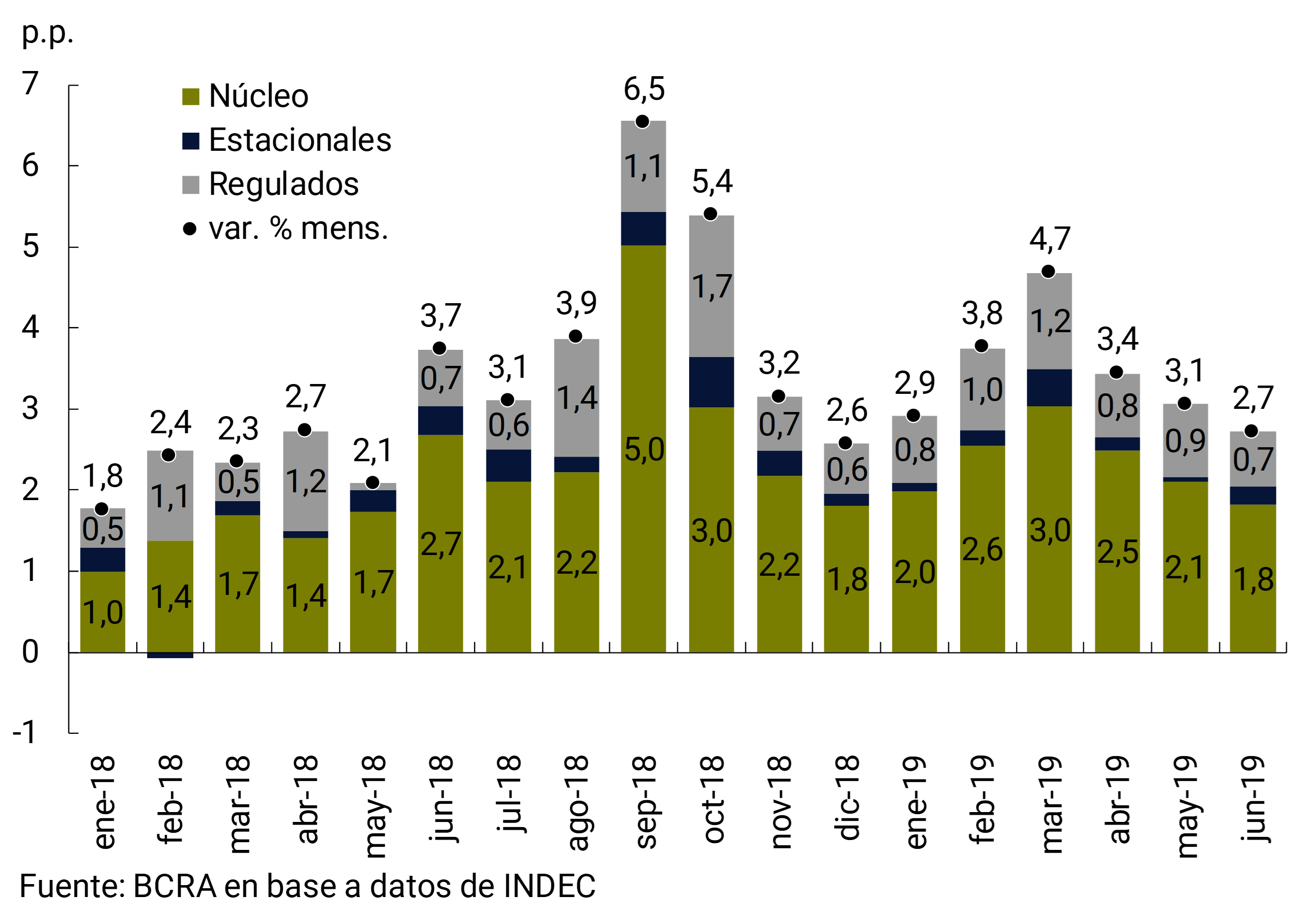
During the second quarter, the performance of the General Price Level reflected to a greater extent the evolution of core inflation, which represents approximately 70% of the CPI basket. The average monthly increase in prices in this category was 3.2%, 0.6 points p.p. lower than that recorded during the first quarter of the year (see Chart 4.2).
Figure 4.2 | National CPI. Contribution by Categories
Both the acceleration of core inflation in the first months of the year and the lower increases recorded in the second quarter were mainly due to the behavior of the prices of goods. During the first quarter, the rise in the prices of goods, which are more tradable, responded to the lagged effect of the exchange rate jump in August and September 2018 and the contemporaneous effect of the depreciation of the peso at the end of the first quarter. The modifications introduced by the BCRA to the monetary-exchange regime in April 2019 reduced the volatility of the exchange rate. Thus, goods went from an average monthly increase of 3.8% in the first quarter of the year to 3.2% in the second quarter.
Figure 4.3 | National CPI. Contribution for Goods and Services
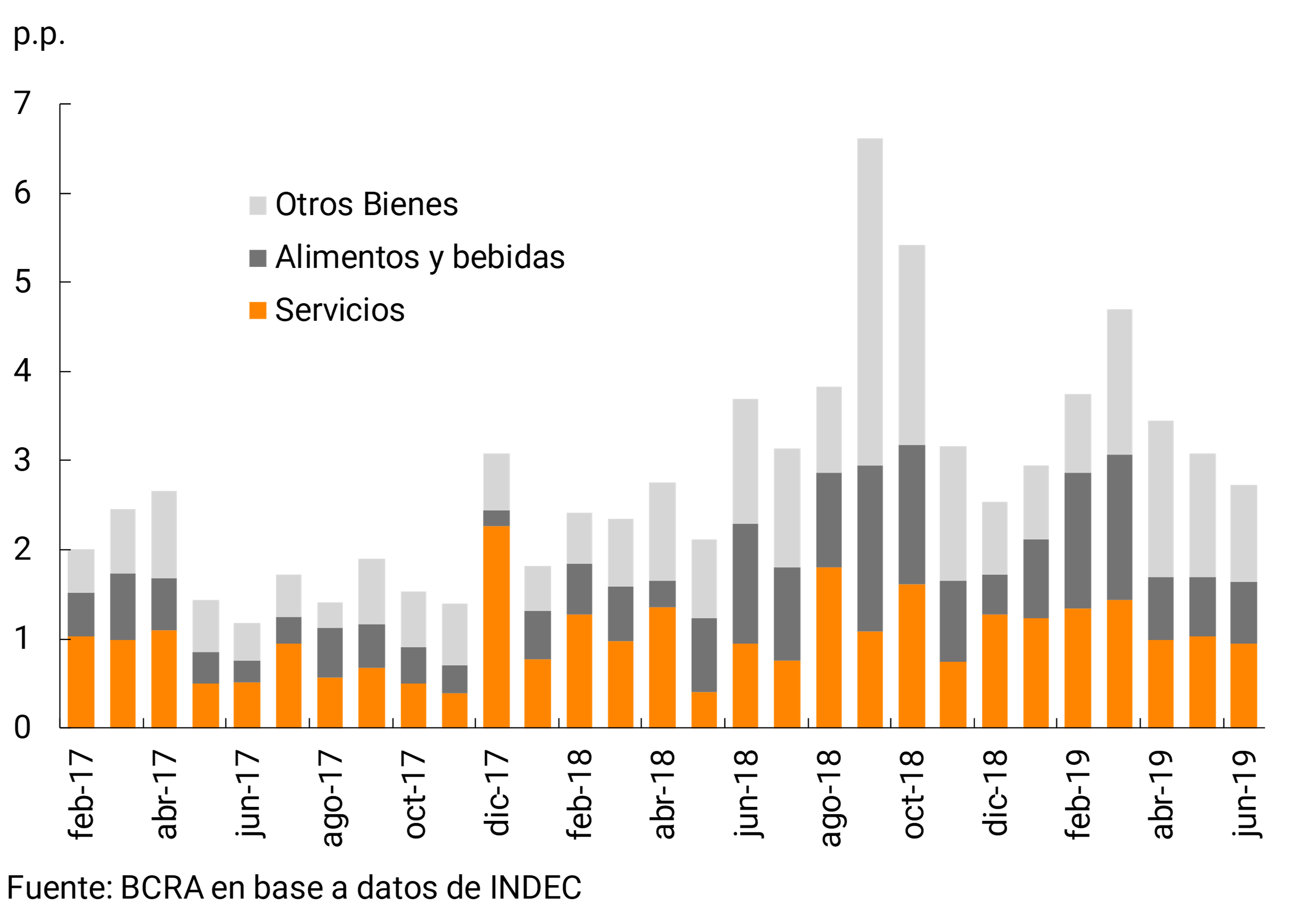
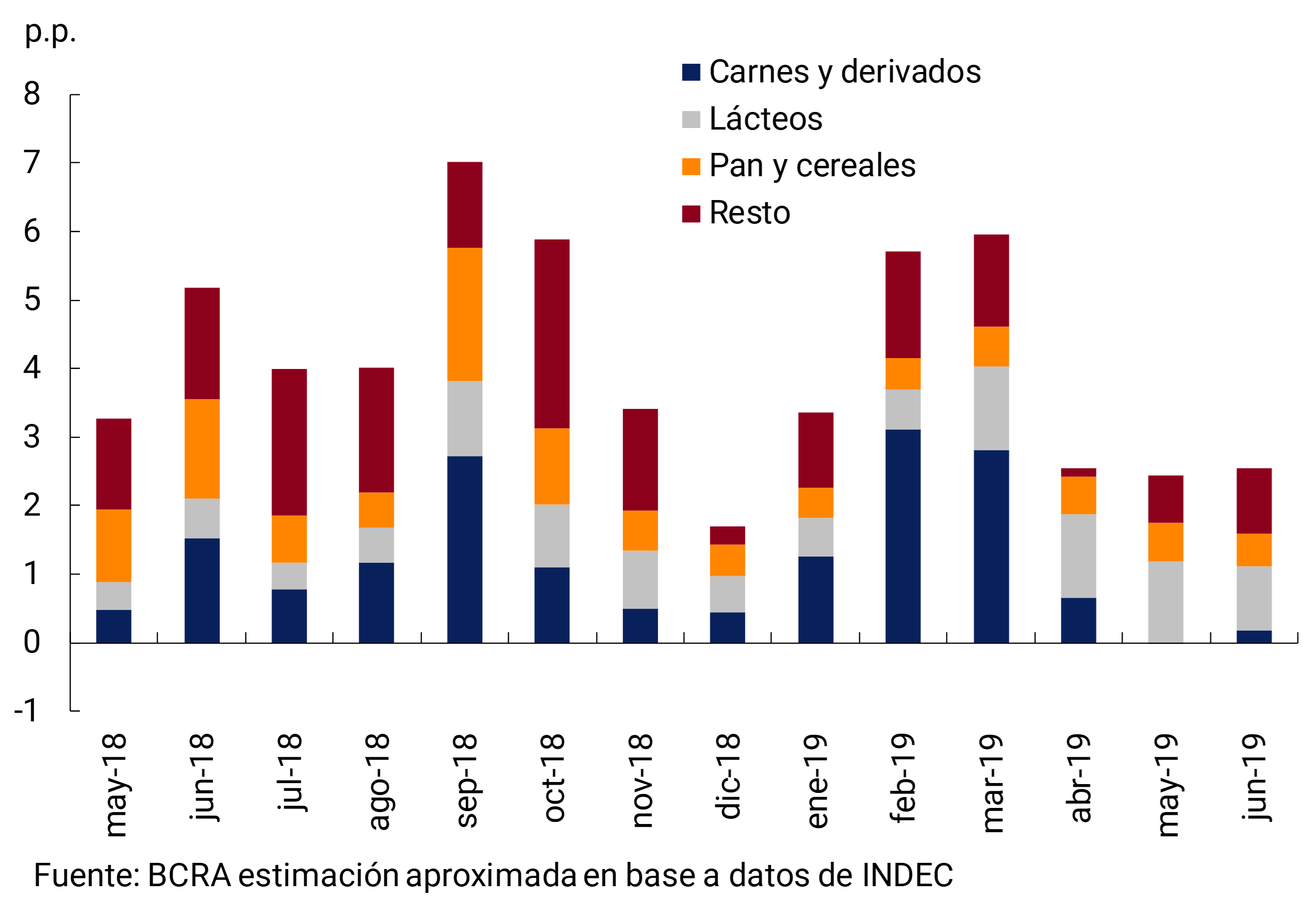
The slowdown in the prices of goods was largely due to the behavior of food and beverages. This category reduced its pace of increase to 2.5% monthly in the second quarter, from 5% recorded between January and March. Within this division, the supply shock that boosted beef prices in the first quarter ceased to operate, taking pressure off food prices. On the contrary, the dairy sector continued to be affected by the supply restrictions verified since the middle of last quarter. The prices of these products continued to grow at higher rates than other foods, with increases of close to 7% per month since March. Dairy price dynamics only partially offset the slowdown in meat prices. Finally, prices of other goods (i.e., goods excluding food and beverages) have gradually slowed since May, in line with lower nominal exchange rate volatility (see Figure 4.3 and Figure 4.4).
Figure 4.4 | National CPI Food and beverages. Contribution by major components
As anticipated in the previous IPOM, the increases in the prices of regulated products were strongly concentrated in the first part of the year. In the second quarter of the year, the prices of regulated products at the national level reduced their average monthly rate of change to 3.3%, 0.9 p.p. below the figure for the first quarter. However, the behavior was not homogeneous at the regional level, with greater increases in the rates of regulated vehicles in the Northwest compared to those registered in the first quarter. The impetus came from the elimination of the social tariff on electricity in some provinces of the region and from provincial increases in the water tariff.
In mid-April, the National Government announced that there would be no new increases in the rates of public services (electricity, gas and public transport) beyond what was already announced. This measure only reaches those rates that are under the orbit of the national executive power, so the components subject to provincial/municipal regulation could be modified in the coming months. Still, the utility rate corrections have been largely completed.
The rest of the regulated goods and services, i.e. excluding public services, continued to adjust in the second quarter. Fuels for vehicles averaged increases of around 4%, influenced by lagged effects of the increase in the exchange rate and tax corrections. The quotas of prepaid medicine evolved in line with the parity of the sector. Educational services continued to increase after March, although they averaged more limited increases. Fixed and mobile telephony services also had updates in their rates between April and June.
Finally, seasonal goods and services also showed a slowdown in their prices in the second quarter, with lower rates of increase than the rest of the components. In fact, the average monthly rate for the second quarter was 1.6% (-1.0 p.p. compared to the first quarter), practically half the rate of increase of the General Level (3.1%). Thus, the set of these items continued to lose relative share in the CPI basket.
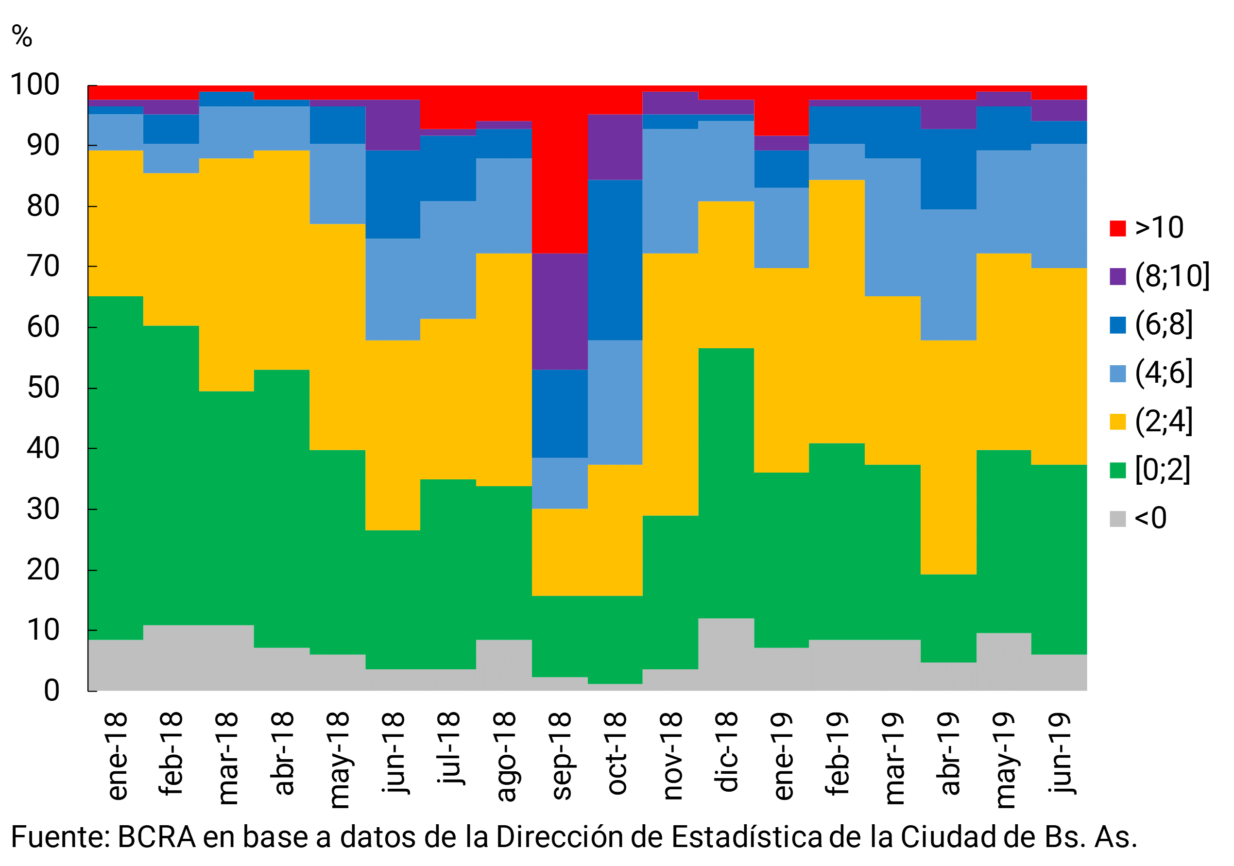
The CPI of the City of Buenos Aires showed a relatively similar behavior to that of INDEC in the accumulated between the end of last year27 , although with some differences in the monthly variations. These responded in general terms to questions related to the composition of the basket, assigning the City’s a greater weight to Services. The similarities in the cumulative behavior allow the data from the City of Buenos Aires to be used to analyze the diffusion and magnitude of price increases. Using the classification by purpose of expenditure, at the maximum level of disaggregation available28, it was observed that as of May the proportion of classes with monthly variations of less than 2% increased. Meanwhile, the proportion of classes with increases of more than 6% decreased. Despite this improvement, price increases are widely disseminated and the distribution of variations still continues to concentrate a high density in values higher than those of the beginning of 2018 (see Figure 4.5).
Figure 4.5| IPCBA. Dissemination of monthly price variations at class level
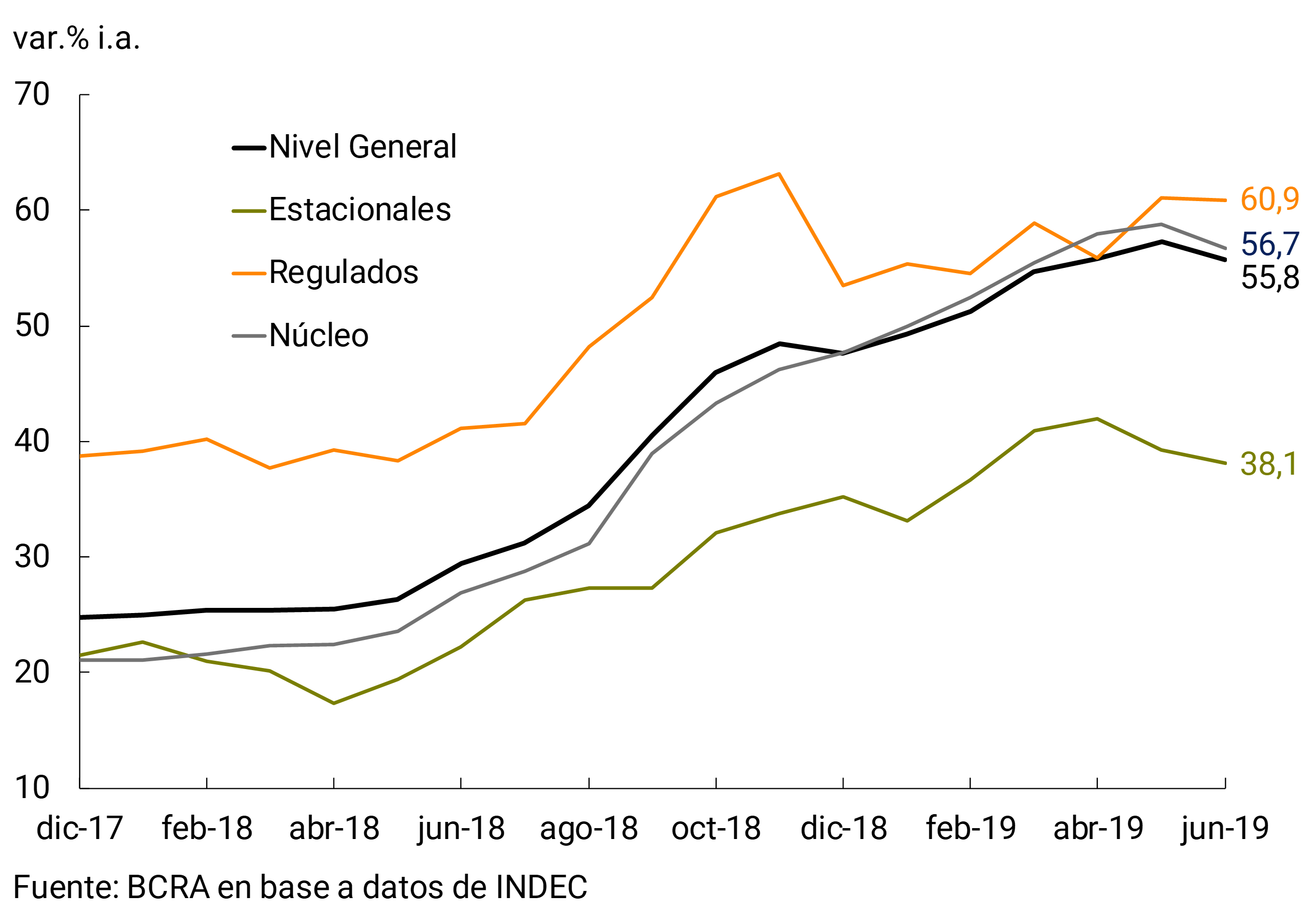
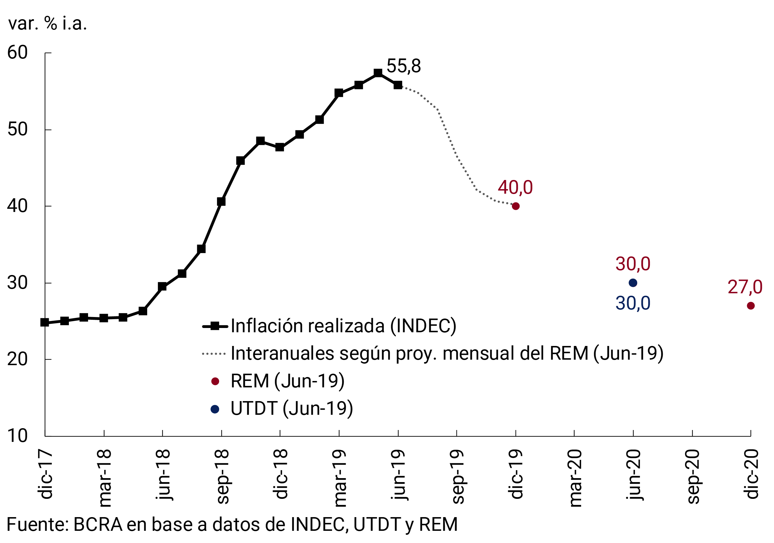
In the second quarter of the year, retail prices continued to grow in year-on-year terms until May, and then exhibited a moderation in the pace of increase. The National CPI registered a 55.8% YoY increase in June, 1.5 p.p. below the peak of May. The year-on-year trajectory of the core component marked an increase of 56.7% y.o.y. in the same period (-2.1 p.p. less than in May). Meanwhile, regulated goods and services grew in year-on-year terms above the rest of prices (60.9% YoY), continuing the process of adjustment of relative prices (see Figure 4.6).
Figure 4.6 | CPI. Year-on-year trajectories by category
Wholesale prices continued to accelerate in monthly terms from March to May in line with the significant increases in the exchange rate between mid-March and the end of April. In June, the fall in the nominal exchange rate anticipates a significant slowdown in wholesale prices, in line with what has happened with consumer prices (see Figure 4.7).
Figure 4.7 | IPIM. Monthly Changes by Division
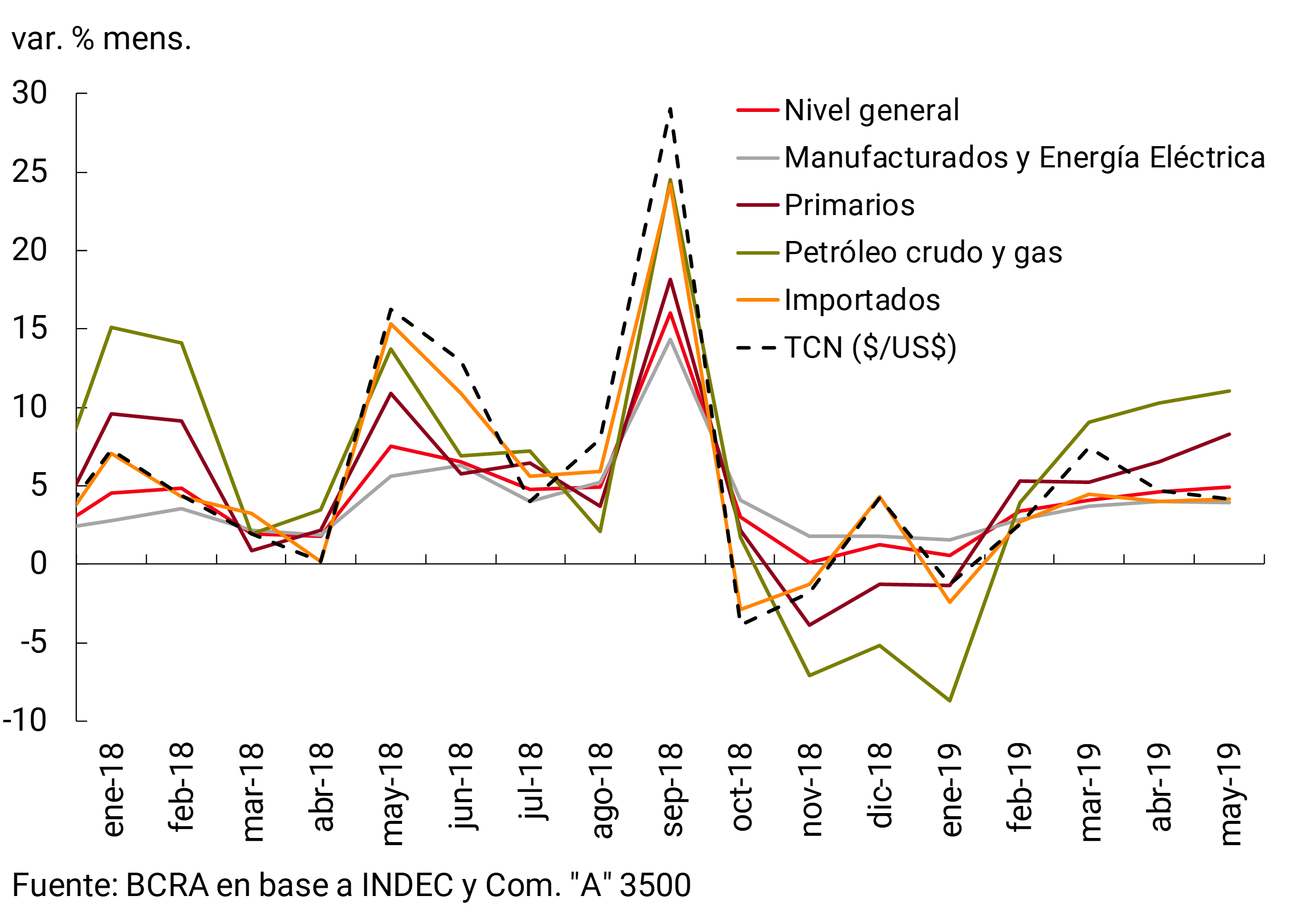
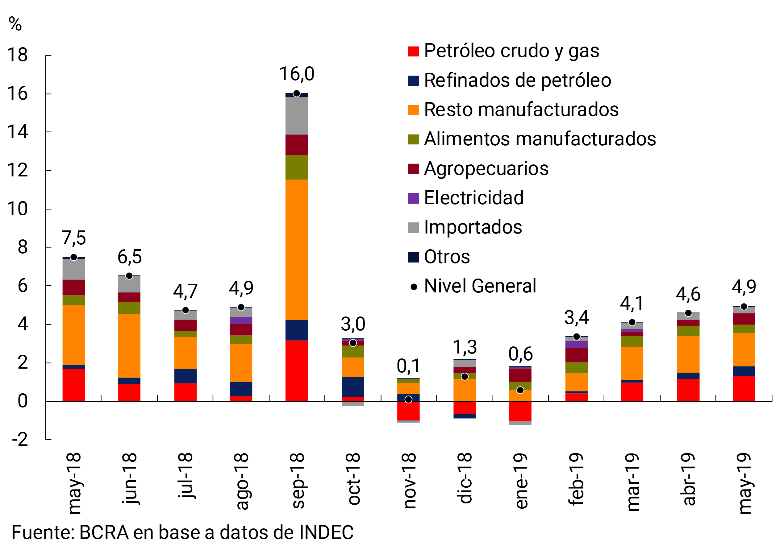
Between April and May, wholesale prices were also affected by increases in international prices of primary products. In the two months, the IPIM averaged a 4.8% monthly increase, 2.1 p.p. above that of the first quarter of the year. In terms of contributions, the largest contribution to the acceleration came from the Crude Oil and Gas component, which averaged increases of around 10% in the two months. This component synthesized the rise in the international price of oil, the depreciation of the exchange rate and the rise in the domestic price of gas at the wellhead. This dynamic was also reflected in refined petroleum products, which, together with chemical substances, contributed to the monthly acceleration of the general level of wholesale prices. To a lesser extent, the rise in international prices of agricultural commodities (cereals and oilseeds) contributed in the same way (see Figure 4.8).
Figure 4.8 | IPIM. Incidents on the General Level
Wholesale food prices moderated compared to the first quarter of the year, but continued to make a significant contribution to the increase in the general level. Producer food prices showed a similar evolution to that of consumer prices. The quotations of live cattle showed more limited variations in April and May, after the shocks that affected these prices in the first months of the year. Meanwhile, vegetable prices fell 17% in the April-May two-month period, helping to take pressure off agricultural prices. Within manufactured products, the prices of meat products remained stable between April and May, after a cumulative increase of 19% in the first quarter. Dairy products averaged monthly increases of 7.3% between April and May, 1.7 p.p. above the average rate of the first quarter. The dynamics of dairy prices partially offset the slowdown in meats, postponing the slowdown in wholesale food and beverage prices until May.
Between April and May, wholesale prices, both primary and manufactured, showed rates of increase that were above those of retail prices, unlike what happened during the first quarter of the year. In this context, the evolution of retail marketing margins29 stabilized, which had been recovering since the last quarter of the previous year after having been compressed after the exchange rate depreciation of August and September 2018 (see Figure 4.9).
Figure 4.9 | Ratio between CPI Goods and IPIM Manufactured

In year-on-year terms, wholesale prices accelerated in March and April and then cut their rates of increase in May, showing a similar trajectory to that of the nominal exchange rate. The IPIM marked an average increase of 70.5% in April and May, standing 4 p.p. above the year-on-year rate of change of the first quarter of the year. The appreciation of the nominal exchange rate in June anticipates a slowdown in wholesale prices, given their high sensitivity to the price of the dollar due to its high component of “tradables” (see Figure 4.10).
Figure 4.10 | IPIM. Year-on-year rates of change

4.2 The temporal distribution of wage increases was more uniform than in previous years
In the second quarter of the year, according to data from the Ministry of Production and Labor (MPyT), nominal wages in the formal private sector continued to accelerate in year-on-year terms. Wages in real terms stabilized in the first part of the year and would begin to show a recomposition starting in May (see Figure 4.11).
Figure 4.11 | Evolution of nominal wages and retail prices
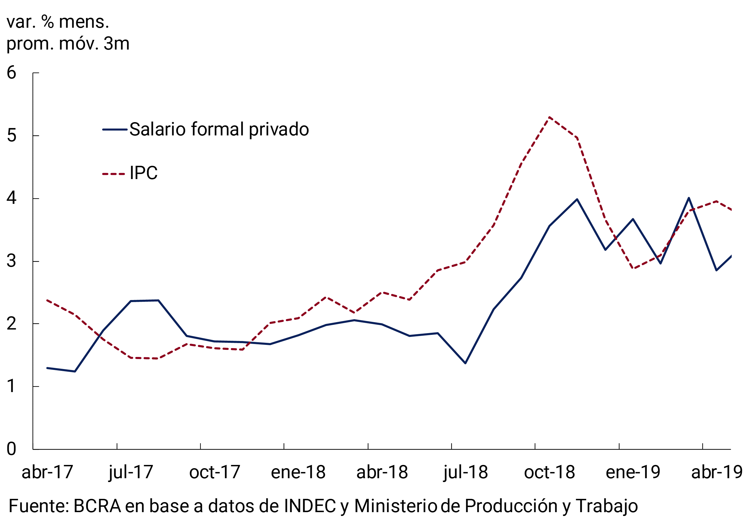
In 2019, the parity negotiations showed greater diversity compared to other years. The agreements contemplated a greater number of tranches, adjustments for inflation and eventual instances of revision of the contracts. Most of the unions negotiated an annual guideline of around 30%, to be integrated into several quotas (between 2 and 6 tranches). Other agreements were structured on the basis of quarterly adjustments, conditional on the evolution of the CPI30. This diversity in the way wages were negotiated resulted in a relatively more heterogeneous distribution (between unions) of wage increase brackets. This behavior was also contributed by the payment, in some cases, of compensatory sums corresponding to 2018. As a result of this heterogeneity, the temporal distribution of wage increases at the aggregate level was more uniform than in previous years in which there was a high concentration of increases in a few months.
Considering the structure of increases agreed in the collective bargaining agreements and if the market’s expectations of a moderation in inflation are met, real wages would improve throughout the second half of the year.
Outlook: The market continues to anticipate a slowdown in monthly inflation rates for the coming months.
As a result of the inflationary acceleration in the first quarter, and in order to prevent it from feeding back into future inflationary expectations, the COPOM decided to reinforce the bias of its monetary policy as of April (see Chapter 5. Monetary Policy). The measures adopted by the BCRA were effective in reducing exchange rate volatility. This, added to the fact that most of the correction in public service rates has already taken place, suggests that inflation would continue to fall in the coming months.
The REM for June anticipates that inflation, both general and core, would register a moderation in the second half of the year as it would be below the average for the second quarter. The REM expects an average monthly variation of 2.3% for the general level and 2.5% for core inflation for the period from June to December (see Figure 4.12).
Figure 4.12 | REM monthly inflation expectations for the second half of 2019

Given the inflation observed in the first six months of the year, market analysts project a rate of increase in prices of 40% y.o.y. as of December 2019. If this scenario is fulfilled, this year’s inflation would be almost 7 p.p. below last year. REM analysts predict a year-on-year growth in prices of 30% for July 2020 and 27% for December of the same year. Thus, according to the REM, the disinflation process would continue both throughout the current year and the next. Along the same lines, the median of the UTDT Inflation Expectations survey, which reflects household inflation expectations twelve months ahead, fell 10 p.p. in May and remained at 30% y.o.y. in June. Meanwhile, the average value of inflation twelve months ago went from 40.8% to 34.5% (see Figure 4.13).
Figure 4.13 | Year-on-year inflation expectations
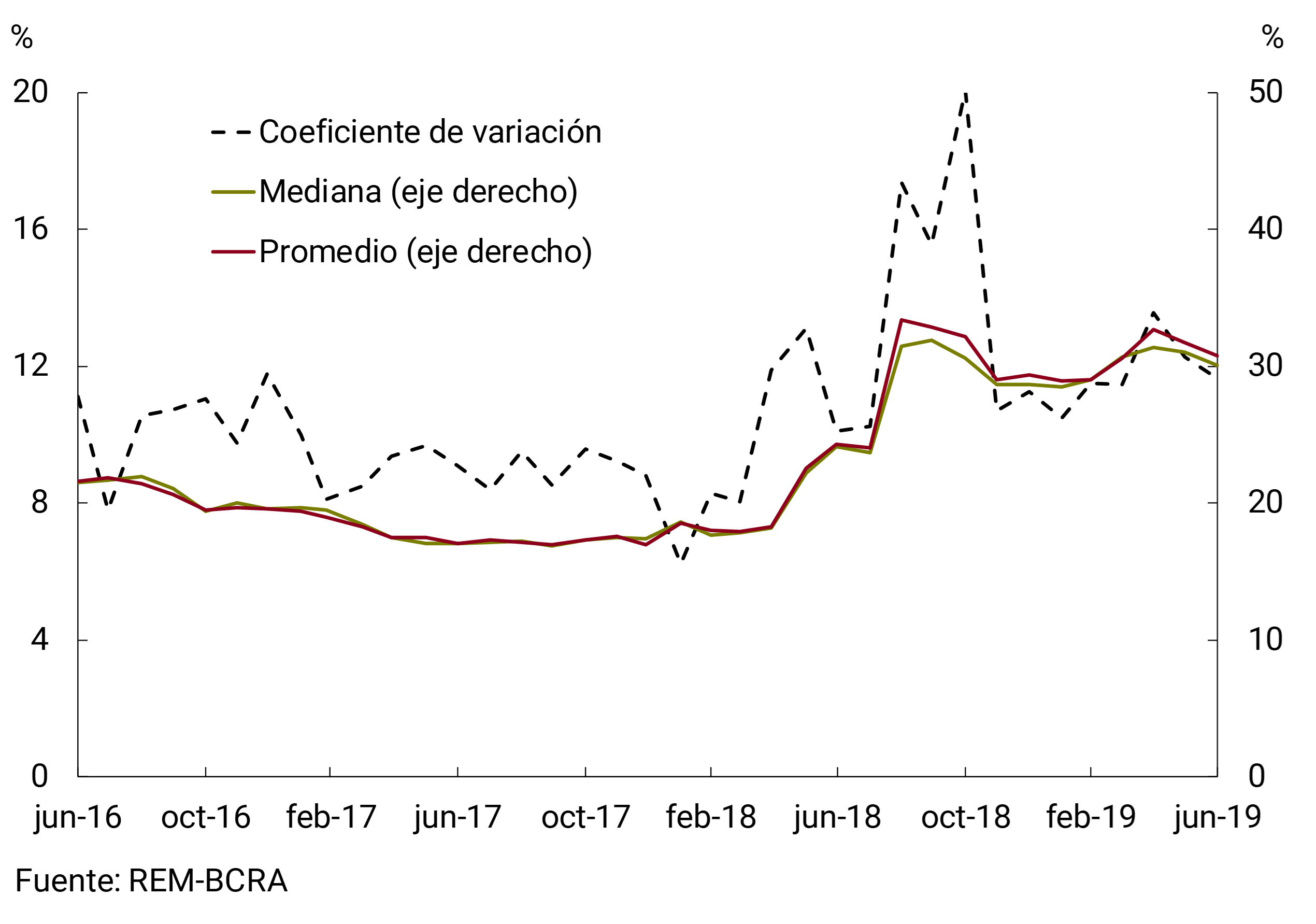
On the other hand, the dispersion of the REM’s inflation forecasts remained around the values of recent months, although it continues to be higher than that recorded during periods of lower inflation. Specifically, the coefficient of variation of the responses for general inflation over the next twelve months stabilized at values close to 12%, almost 8 p.p. below the October peak and approximately 4 p.p. above the 2017 average (see Figure 4.14).
Figure 4.14 | CPI General level Next 12 months. Coefficient of variation, median and average
5. Monetary policy
Given the reappearance of exchange rate instability in March and its disruptive effect on the ongoing disinflation process, the Monetary Policy Committee (COPOM) announced in April modifications to its foreign exchange intervention scheme: it set the growth of the limits of the exchange reference zone (formerly called the non-intervention zone) at zero until the end of the year and provided for the possibility of selling foreign currency even when the exchange rate is above the lower limit of the exchange rate reference zone. In the same sense, the COPOM reestablished the floor of the reference interest rate (LELIQ rate). In the current monetary scheme, the reference rate is endogenous, that is, it is the one that ensures that the demand for LELIQ is consistent with the monetary base objective. But by guaranteeing a floor, the COPOM gives greater predictability to its evolution. Finally, with the launch of fixed-term operations for non-customers, the BCRA stimulated competition among financial institutions and improved the mechanism for transmitting the reference interest rate to the rest of the interest rates in the economy.
The measures adopted and the maintenance of a restrictive monetary policy, in a context of better international conditions, allowed inflation to decrease as of April and stabilized inflation expectations and the foreign exchange market. In an environment of lower nominal volatility and low inflation expectations, the nominal interest rate of the LELIQ showed a downward trend since the beginning of May, with the real interest rate remaining at high levels in historical terms.
The electoral process usually entails greater financial uncertainty. With these tools, the BCRA will be better equipped to mitigate its impact on nominal variables and thus give greater predictability to price makers.
5.1 Monetary policy in the second quarter of the year
5.1.1 The Central Bank took further steps to reinforce the contractionary bias of monetary policy
The high levels of inflation in February and March and the increase in exchange rate volatility from February onwards had led the Monetary Policy Committee (COPOM) to take measures in mid-March to strengthen the monetary scheme (see Section 3 for a description of how the scheme operated in its first nine months). Thus, it extended the objective of zero growth of the monetary base until the end of the year, eliminating the seasonality adjustment planned for June (maintaining the 6.3% adjustment of December), and set the target at the level reached during February ($1,343.2 billion), making permanent the overfulfillment of the target reached in that month. 31
Given the persistence of exchange rate volatility, the COPOM took additional measures in April to reinforce the restrictive bias of monetary policy and prevent further shifts from the exchange rate to the inflation rate.
Thus, the COPOM decided to leave the limits of the non-intervention zone (ZNI) constant at $39,755 and $51,448 for the rest of the year (see Figure 5.4). 32 It also established that no foreign exchange purchases would be made in the event that the exchange rate was below the lower limit of the ZNI until June 30, which guaranteed that the monetary base target would not increase for this reason (later, this was extended until July 31). In the event that the exchange rate is above the upper limit of the ZNI, the Central Bank would maintain its intervention mechanism of selling up to US$150 million per day through auctions and the monetary base target would be reduced with such sales.
Later, the COPOM decided that the Central Bank could make sales of foreign currency even when the exchange rate was within the ZNI, which was renamed the exchange reference zone (ZRC). The amount and frequency of these interventions became dependent on market dynamics. 33 It also defined that the daily sale of foreign currency will increase from US$150 to US$250 million if the exchange rate is above $51,448, although additional sales may also be made to counteract episodes of excessive volatility. In all cases, the amount of pesos resulting from these sales will be discounted from the monetary base target, reinforcing the contractionary bias of monetary policy in these scenarios.
Additionally, with the aim of maintaining a restrictive monetary policy and showing caution in the face of possible episodes of uncertainty, the COPOM announced a floor of 62.5% per year for the reference interest rate, which was in force during the April-June quarter and was reduced to 58% annually in July.
To promote competition among financial institutions and improve the mechanism for transmitting the reference rate to the passive rates of financial institutions, the Central Bank allowed bank customers to make fixed-term deposits in pesos online at any financial institution without having to be customers or carry out additional procedures (see Section 5).34
Finally, in mid-April, the Ministry of Finance began to hold daily auctions for US$ 60 million to cover needs in pesos. These tenders will be carried out to reach a cumulative amount of US$9,600 million in November of this year. 35
5.1.2 The Central Bank met the monetary targets
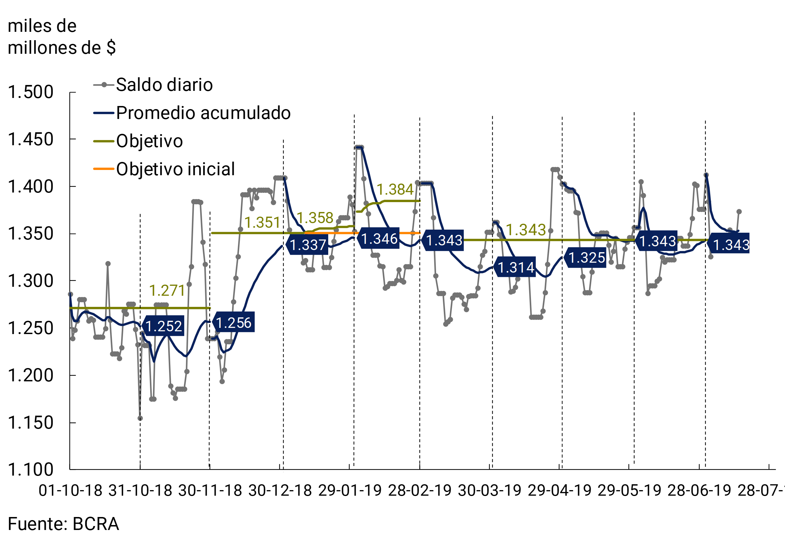
In the second quarter of the year, the Central Bank met its goal of zero growth of the monetary base (WB), accumulating nine consecutive months of compliance (see Figure 5.1). 36 The target throughout the quarter remained at $1,343.2 billion, due to the fact that there were no interventions by the monetary authority in the foreign exchange market. 37
In April, the Central Bank exceeded the target by $18 billion (1.4%), while in May and June compliance was tighter, $591 million (0.04%) and $1,300 million (0.1%), respectively. During May, the increase in the WB was mainly explained by the higher reserve requirements generated by the increase in public sector deposits. To moderate its monetary impact, part of these deposits were transferred by the National Treasury to the Central Bank. At the end of May, a transfer of profits from the BCRA to the National Treasury was made for $77,245 million, an amount equivalent to the interest payment that the latter will have to make to the monetary authority for its holdings of public securities during the rest of the year. This operation had no monetary effect, not even temporarily, since these funds are deposited in the Treasury account at the Central Bank until they are used to make the payment. 39 In June, the fulfillment of the goal was particularly demanding due to the seasonal behavior of the demand for BM, which is increased by the payment of the half bonus and the higher expenses of the winter recess (see Section 4).
Figure 5.1 | Monitoring of monetary base targets
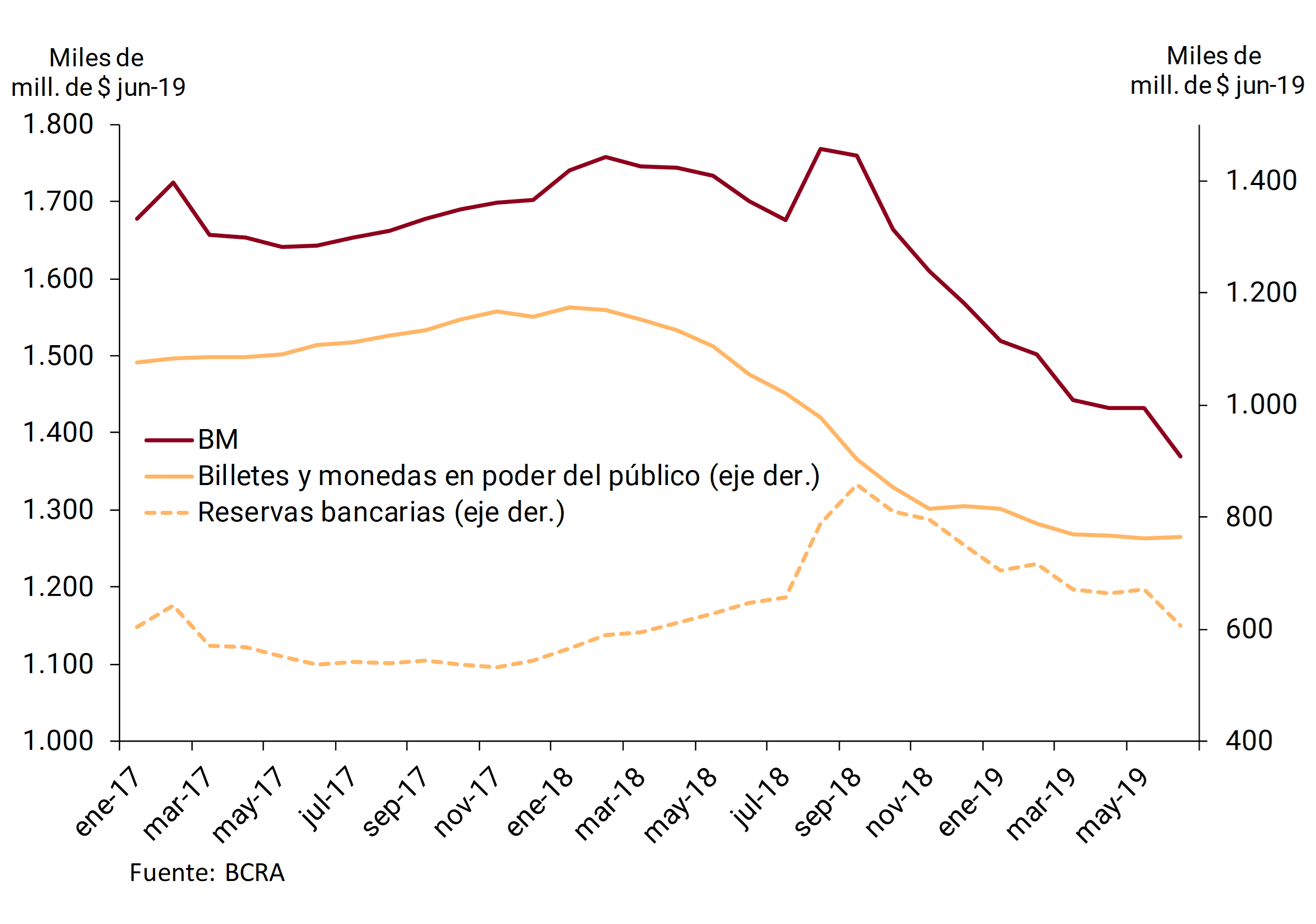
Given the dynamics of inflation in the second quarter of the year, meeting the monetary target continued to imply a significant reduction in the quantity of money in real terms, reflecting the contractionary bias of monetary policy. The World Bank fell 5.0% in real terms without seasonality between March and June of this year and accumulated a real fall without seasonality of 22.2% since the beginning of the monetary scheme in October last year (see Figure 5.2). Currency held by the public contracted 0.8% in the quarter (in real terms without seasonality), moderating its rate of contraction compared to what was observed in previous quarters, while bank reserves showed a greater contraction (-9.9% in the quarter in real terms without seasonality).
Figure 5.2 | Monetary base and its components (in real terms without seasonality)
In July, the monetary base target remained at $1,343.2 billion. During this month, the high seasonality of the demand for working capital continues. In order to allow for better management of liquidity conditions in this period and to help strengthen the transmission of the interest rate of the LELIQ to the rate received by savers, the BCRA decided to reduce the minimum cash requirement on fixed-term deposits by 3 p.p. This represents a reduction in the demand for the monetary base due to reserve requirements of approximately $45 billion that compensates for the seasonal increase in the demand for working capital. In order to maintain the contractionary bias of monetary policy, once this seasonal phenomenon has been overcome, the monetary base target will be reduced as of August to reach $1,298.2 billion in October; this will fully offset the effect of the reduction of reserve requirements. 40
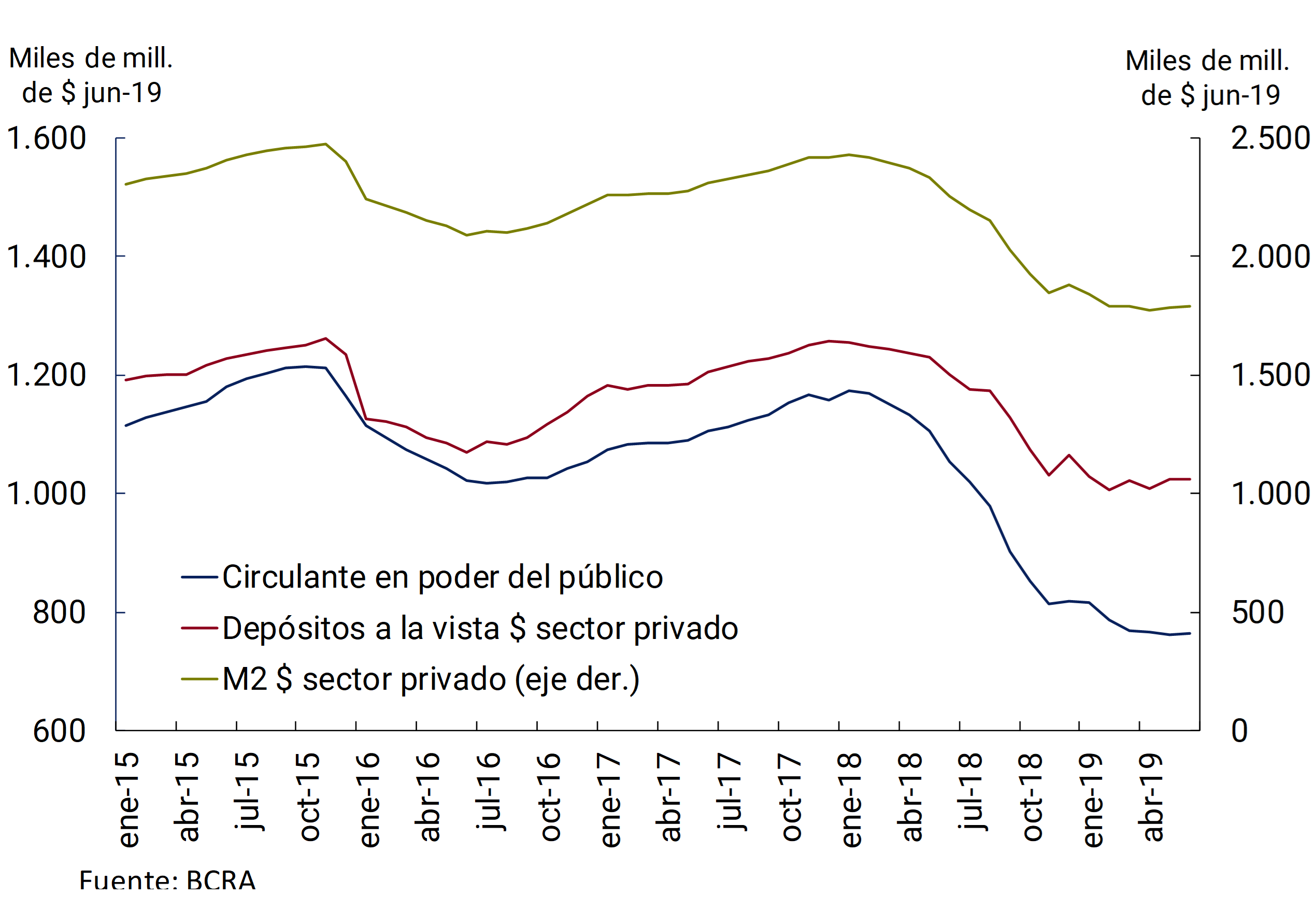
The private M2 monetary aggregate in pesos was stable during the second quarter in real seasonally adjusted terms (reduction of 0.1% per month on average), after the contractionary trend recorded during most of last year (see Figure 5.3). 41 This behavior was mainly a consequence of the stability of demand deposits in pesos in the private sector (current account and savings banks), which did not vary in the period in seasonally adjusted real terms.
Figure 5.3 | M2 in pesos of the private sector (in real terms without seasonality)
5.1.3 Exchange rate volatility was reduced, inflation expectations stabilized, and the interest rate began to fall
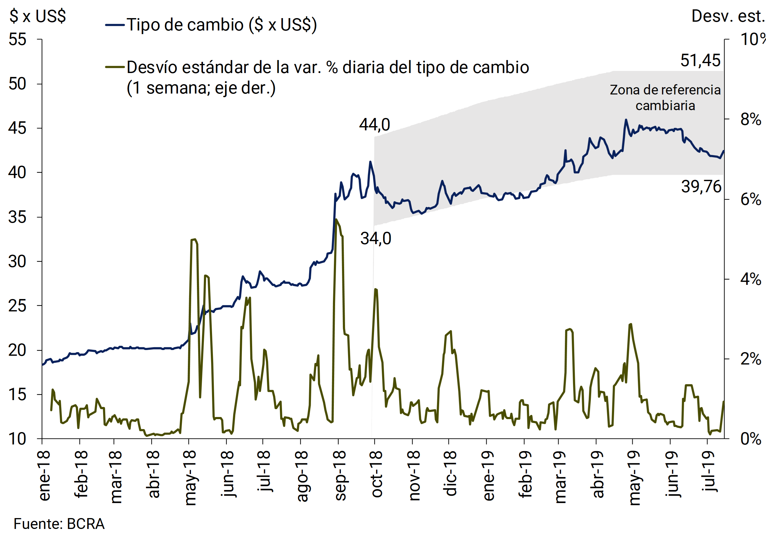
The measures adopted and the maintenance of a restrictive monetary policy, in a context of better international conditions, contributed to the stabilization of exchange rate dynamics. After rising 19 percent between early February and late April, the U.S. currency fell 4 percent through mid-July, while weekly volatility in daily exchange rate changes declined sharply from its peak in late April (see Figure 5.4). At the same time, inflation began to show a downward trajectory since April and inflation expectations stabilized in the May and June surveys (see Chapter 4). 42
Figure 5.4 | Recent exchange rate developments and volatility
When setting a target on the quantity of money, the benchmark interest rate is determined by the demand for liquidity in LELIQ’s daily auctions. If there are increases in inflation expectations or a greater perception of risk, financial institutions demand a higher interest rate to maintain their positions in pesos, which is quickly reflected in the interest rate that arises from LELIQ’s tenders. This reaction of the benchmark interest rate helps to reduce exchange rate volatility and increase the contractionary bias in the face of inflationary surprises.
Thus, in the face of the greater exchange rate volatility in April, the benchmark interest rate increased by 7.2 p.p. to reach 74.1% annually on May 2 (see Figure 5.5). This dynamic of the nominal reference rate implied that the real interest rate has reached a high level in historical terms, which reinforces the contractionary bias of monetary policy (see Figure 5.6). 43 Then, in a context of lower nominal volatility and falling inflation expectations, the nominal interest rate of the LELIQ showed a downward trend until it reached the minimum of 62.5% per annum set by the COPOM for that month in the last days of June. For July, the COPOM decided to reduce the minimum rate of LELIQ auctions to 58% per annum, in line with the drop in inflation observed and that expected by the REM for this month. 44 The interest rate on the LELIQ continued to be gradually reduced until it reached 58.8% per annum on the 15th.
Figure 5.5 | LELIQ interest rate and stock of interest-bearing liabilities in pesos (LEBAC, LELIQ, NOCOM and net passes)
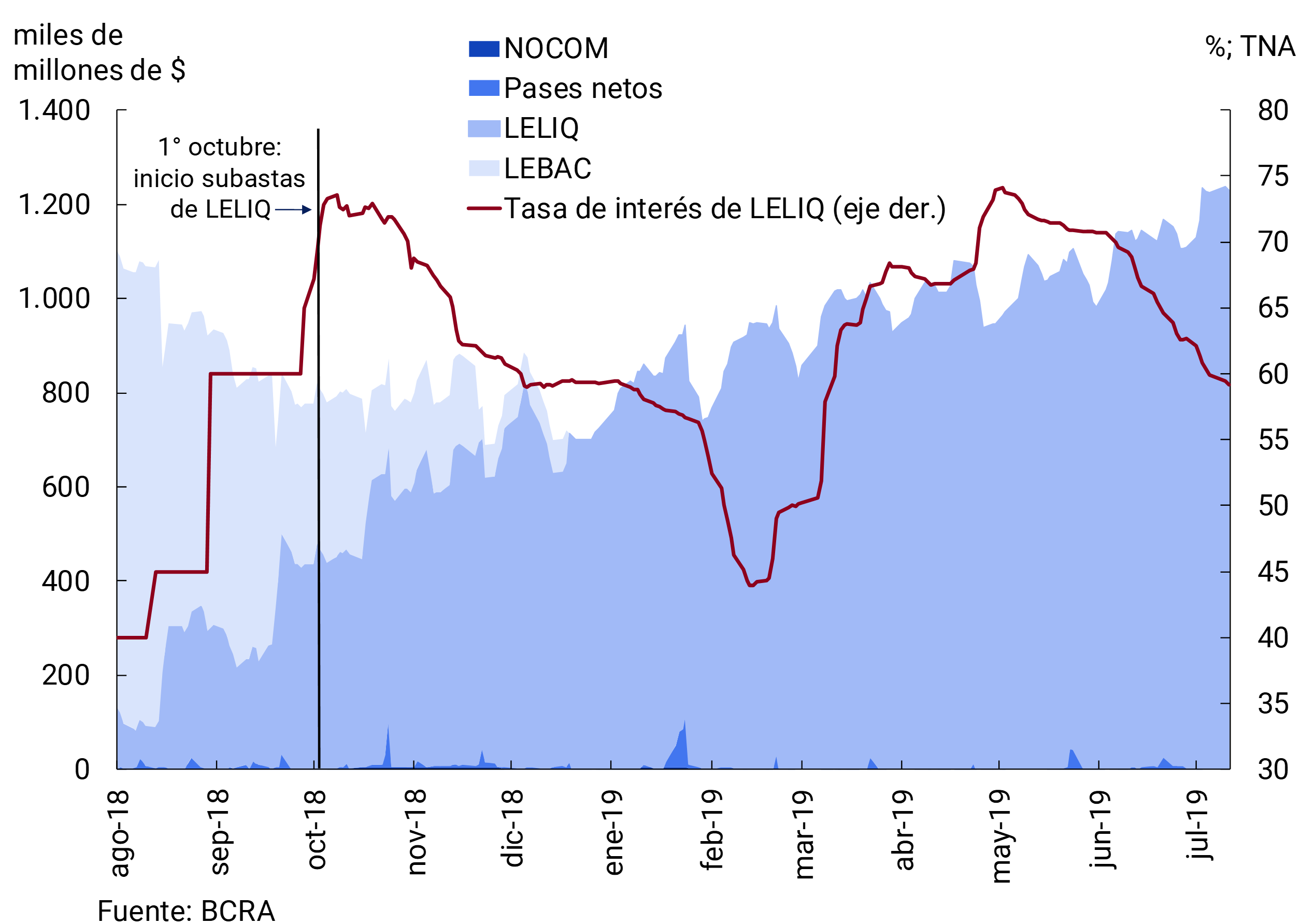
Figure 5.6 | Reference real interest rate (effective monthly rates – ex post)*
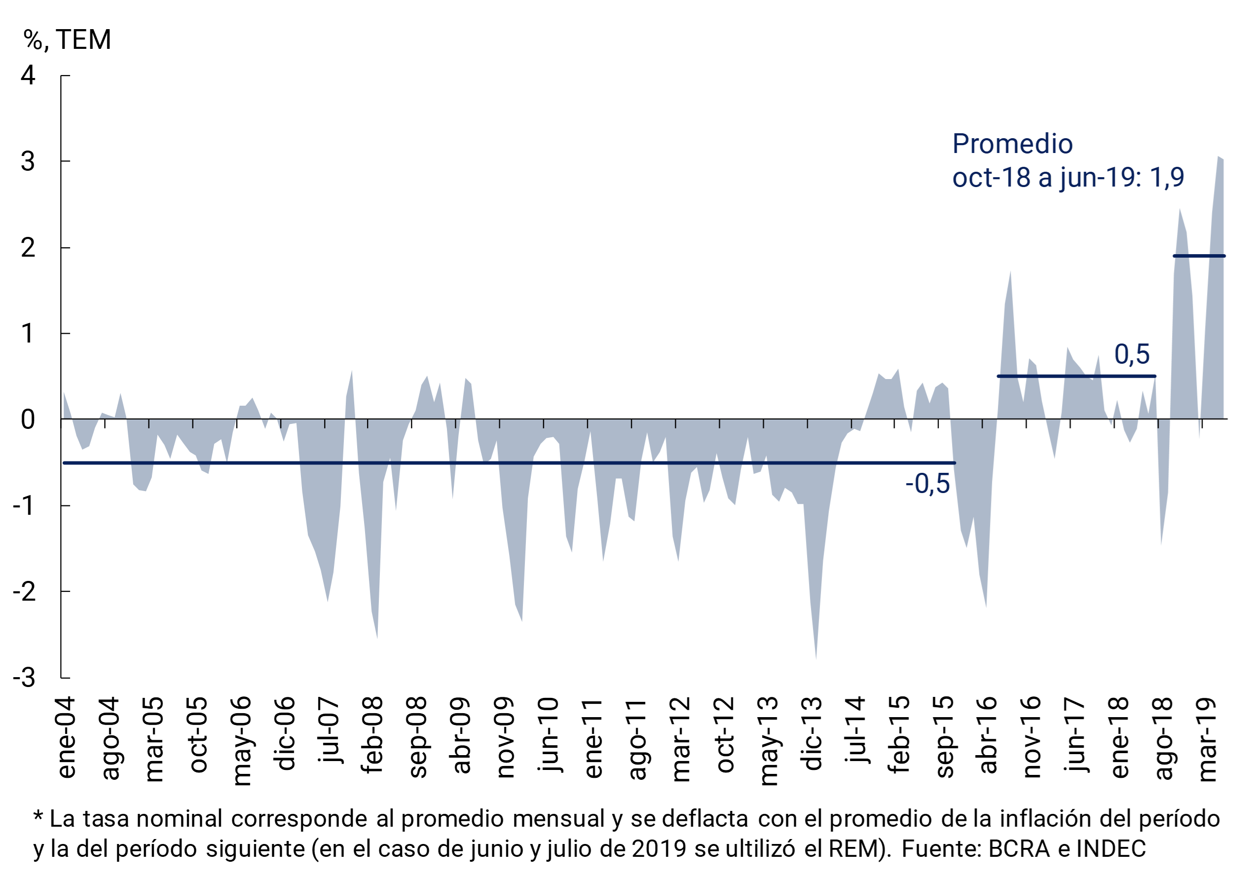
The Central Bank’s interest-bearing liabilities in pesos (LELIQ, NOCOM and net passes) showed an upward trajectory in nominal terms in the second quarter, going from $955.3 billion at the end of March to $1,232.3 billion at the beginning of July (see Figure 5.5). This increase was mainly associated with the accrual of interest and, to a lesser extent, with some foreign currency purchase operations from the National Treasury at the end of June and beginning of July. 45 However, the stock of interest-bearing liabilities was 16% below the peak of $1,459.0 billion reached on March 20 of last year (when LEBACs were included). At the same time, in terms of GDP, these liabilities represented 5.3% in June, compared to 10.6% in March last year, and as a ratio of international reserves they reached 0.40 in June, compared to 1.12 in March 2018 (see Figure 5.7).
Figure 5.7 | Central Bank’s interest-bearing liabilities in pesos (LEBAC, LELIQ, net passes and NOCOM) (in terms of GDP and international reserves)

The evolution of international reserves in the second quarter was mainly explained by the debt operations of the National Treasury and was not related to the Central Bank’s exchange rate policy, since it did not intervene in the foreign exchange market (see Figure 5.8). These Treasury operations included foreign exchange inflows of US$21,997 million as a counterpart to borrowing operations in foreign currency (US$10,830 million from the income from the fourth tranche of the Stand-by arrangement with the IMF, US$1,383 million from disbursements from other international organizations – mainly the IDB and the World Bank – and US$8,785 million for other debt placements). in the face of foreign currency outflows due to payments of debt maturities in foreign currency of US$19,710 million and daily auctions of foreign currency in the market for US$3,000 million. 46 In net terms, these operations accounted for US$1,713 million of the US$1,909 million that fell in reserves in the quarter, which reached US$64,278 million at the end of June. Thus, the ratio of monetary base plus interest-bearing liabilities in pesos to international reserves valued in pesos remained at the lowest levels in recent years, at an average of 0.87 in June compared to 1.94 in March 2018 (see Figure 5.9).
Figure 5.8 | Explanatory factors for the change in international reserves in the second quarter of 2019
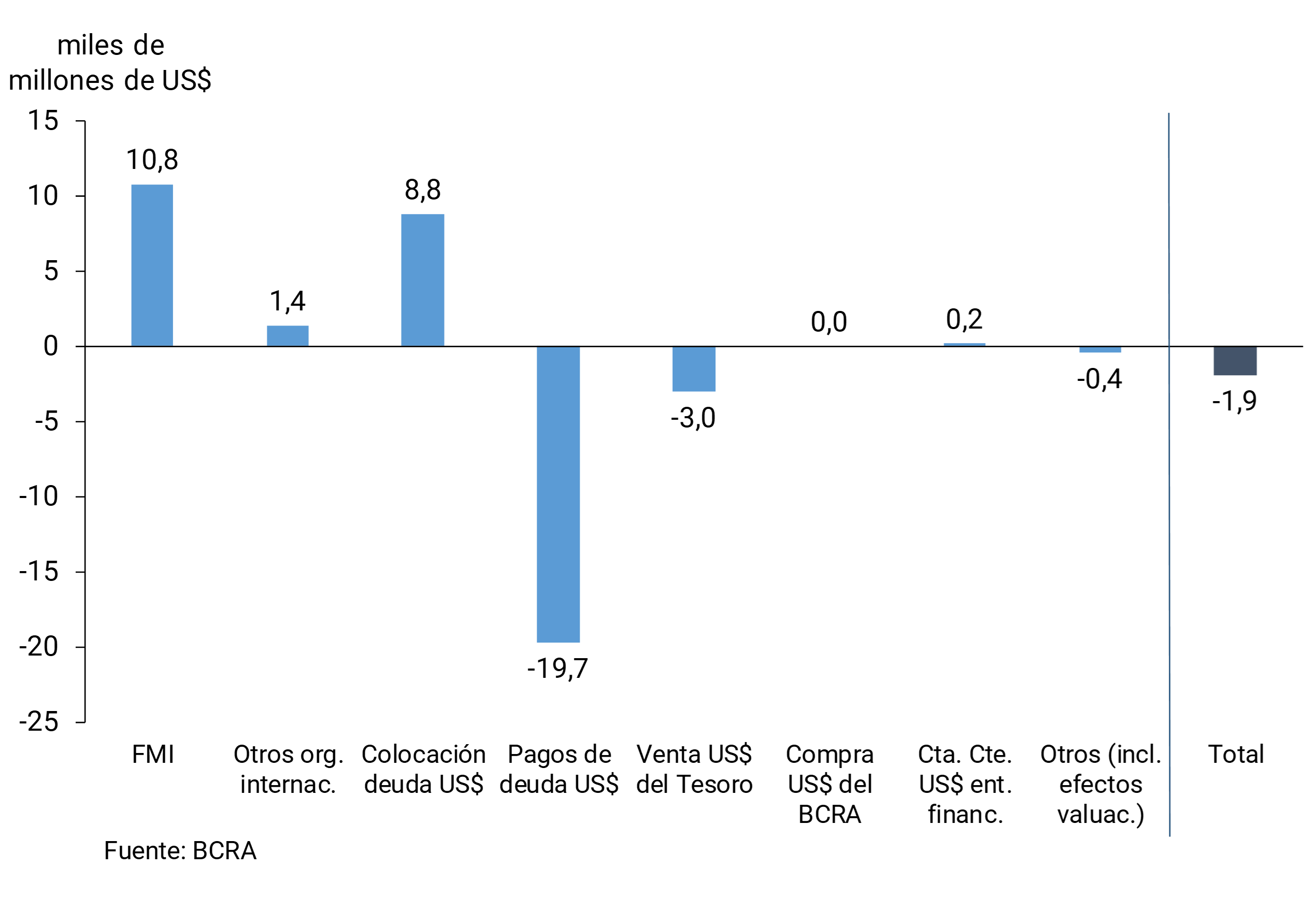
Figure 5.9 | Central Bank International Reserves
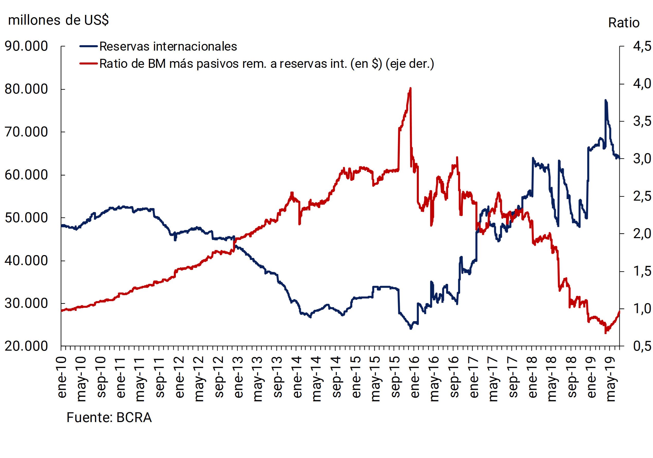
5.1.4 Outlook
The contractionary bias of the monetary scheme will continue throughout 2019 with the fundamental purpose of consolidating the downward trajectory evidenced by the inflation rate in recent months. At the same time, this monetary policy stance allows the Central Bank to be prepared to face possible sources of uncertainty. The disinflation process is expected to be non-linear and gradual, due to inflationary inertia. In this context, the benchmark interest rate is expected to fall gradually, only to the extent that expected inflation decreases and no new volatility events arise.
Although this scenario of normalization of the economy could be affected by some risks, mainly linked to a new episode of volatility in global financial conditions or to the usual uncertainty of the electoral processes in Argentina, the Central Bank is in a better position to moderate the impact of these risks on the economy.
On the one hand, the monetary authority’s balance sheet is more solid. The Central Bank’s stock of interest-bearing liabilities in pesos is at limited levels both in terms of GDP and international reserves, following the LEBAC cancellation program in the second half of last year (see Figure 5.7). In a context in which the public sector is adjusting its accounts, one of the main factors of creation of the monetary base that operated in the past, such as transfers to the Treasury, has been eliminated, which reduces the need for sterilization by the monetary authority. Even assuming a scenario in which the interest rate on the LELIQ remained at levels of 60% per year, the weight of interest-bearing liabilities in GDP would reach 6.0% in December 2019, which would be 4.6 p.p. lower than the peak recorded in March last year (see Figure 5.10).
Figure 5.10 | Central Bank’s interest-bearing liabilities in pesos under a constant interest rate scenario (in terms of GDP)
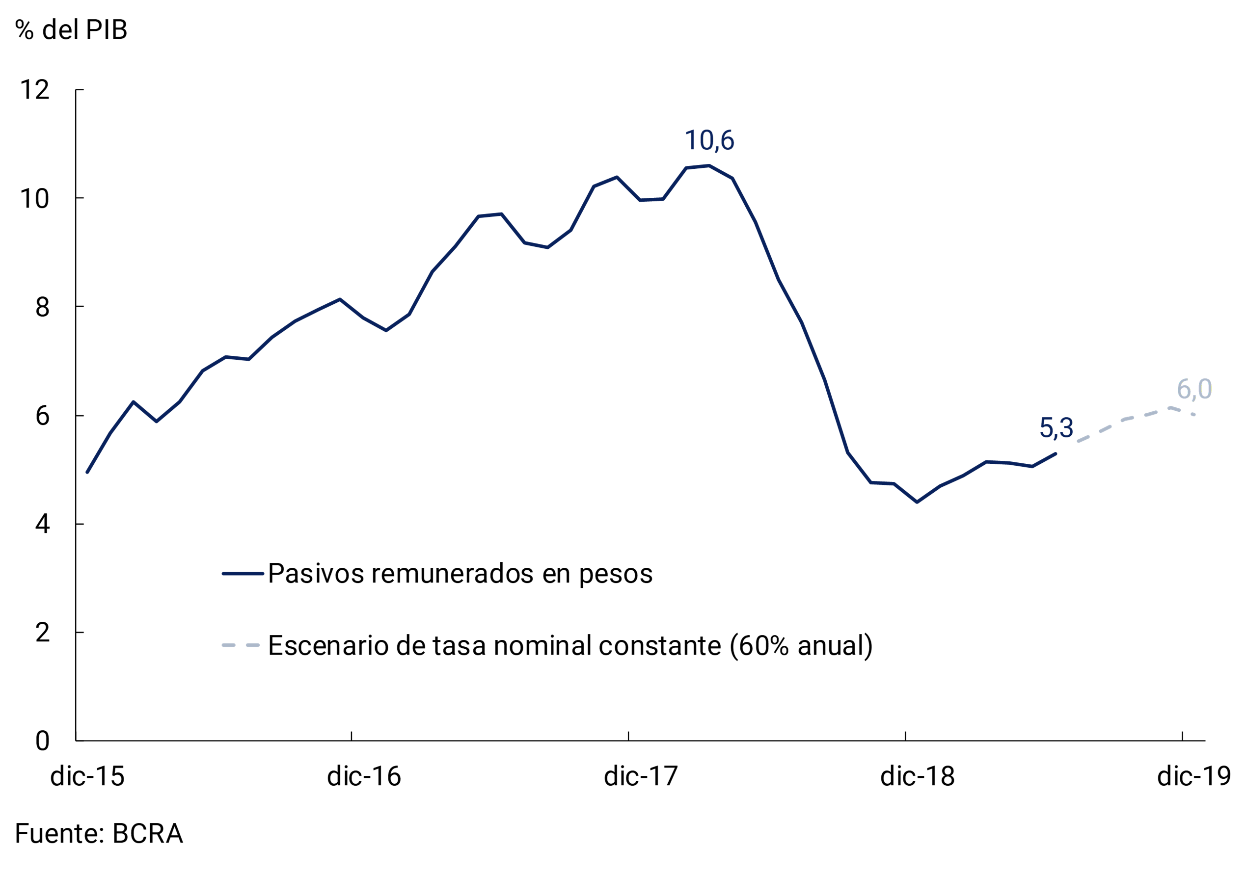
On the other hand, the real exchange rate is about 50% above the level it was before the unification of the foreign exchange market in December 2015 and remains at levels similar to those of the end of 2011, when the economy registered a current account balance close to equilibrium (see Figure 5.11). This level of the real exchange rate is contributing to the adjustment of the external accounts. In fact, the current account deficit in the first quarter of 2019 (seasonally adjusted and annualized) was 2.2% of GDP, compared to 6.5% in the second quarter of 2018, which implies an adjustment of 4.3 p.p. in just three quarters.
Figure 5.11 | Multilateral Real Exchange Rate
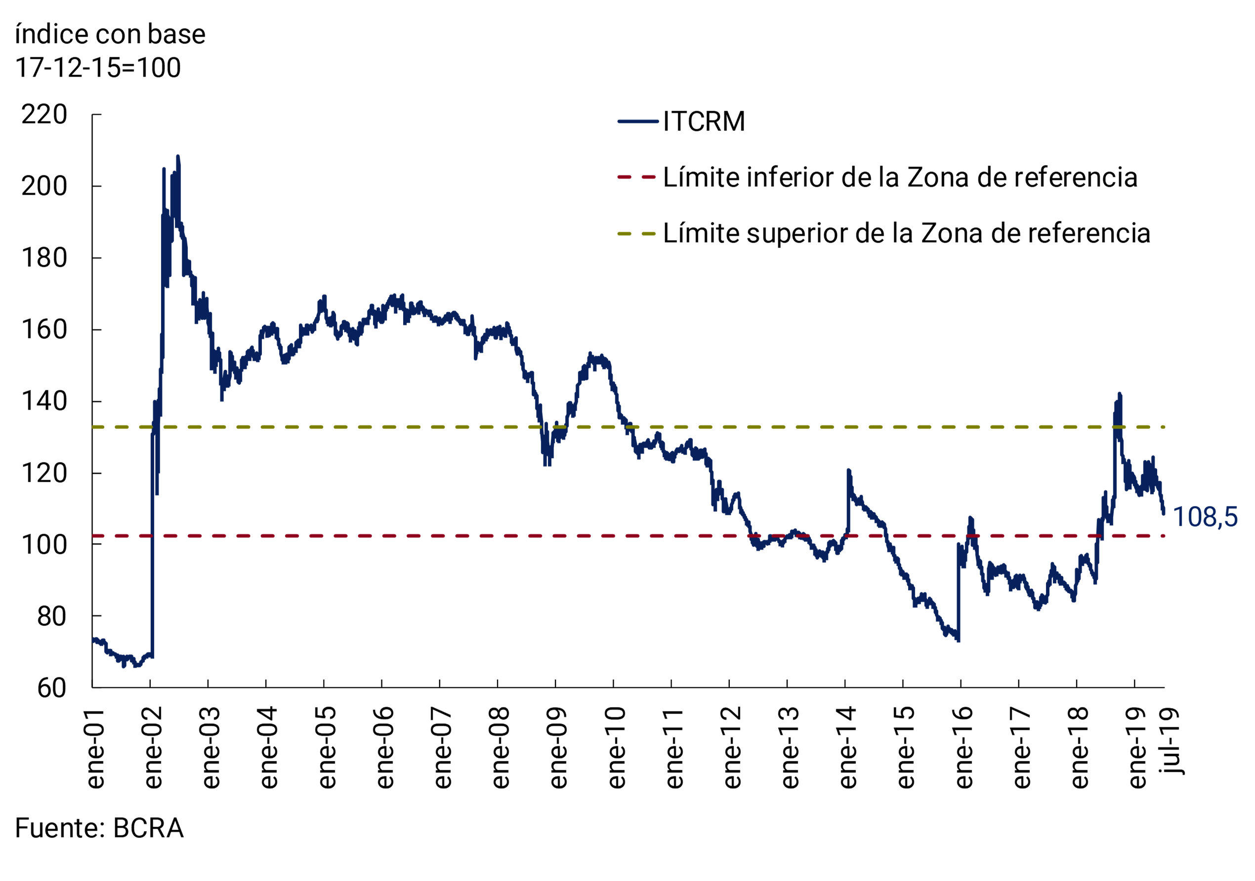
Finally, the monetary aggregates in pesos of the private sector are at the lowest levels of the last fifteen years, which mitigates the magnitude of an eventual episode of dollarization (see Figure 5.12). In addition, the monetary authority has greater degrees of freedom to intervene in the foreign exchange market in the face of episodes of disruptive exchange rate volatility together with an adequate stock of international reserves (see Figure 5.9).
Figure 5.12 | Private sector monetary aggregates in pesos
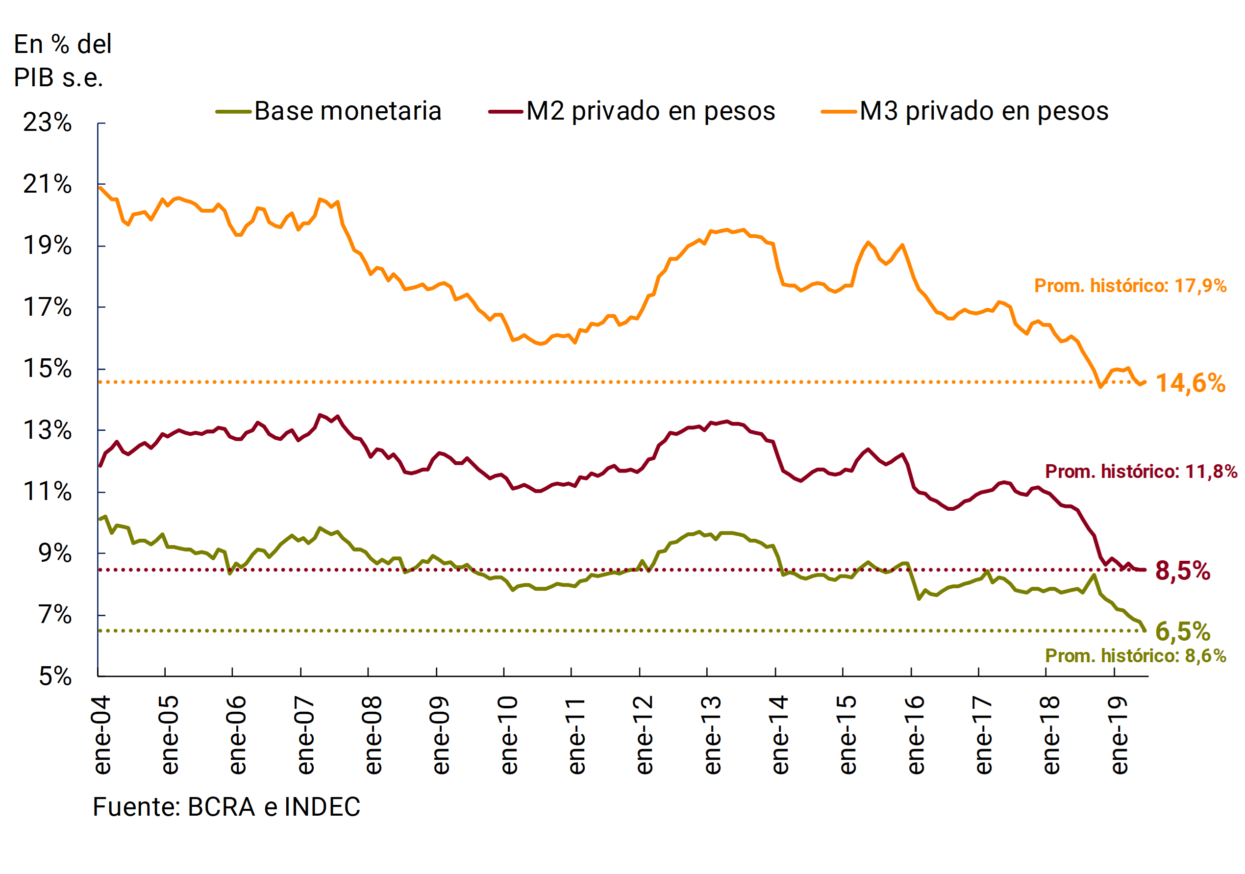
5.2 The financial system in the second quarter of the year
The lending and passive interest rates of the financial system followed the movements of the reference interest rate (LELIQ rate), showing a downward trend since the beginning of May. Spreads were compressed as part of the measures adopted by the BCRA to promote competition in the financial system (see Section 5). Credit to the private sector continued to contract, although at a slower pace than in the previous quarter, while deposits showed strength in the face of the greater exchange rate volatility recorded in April.
5.2.1 Interbank rates accompanied the movements of the benchmark interest rate
During the second quarter of the year, money market interest rates accompanied the rise in the reference rate in April, as well as its subsequent decline during the months of May and June (see Figure 5.13). The 1-day third-party pass rate fell by 5.2 p.p. between the end of March and June, reaching 56.6% year-on-year, and maintained its spread with the LELIQ rate. While the 1-day call rate fell 0.2 p.p. in the same period, reaching 61.6% annually, and gradually reduced its spread with the reference rate, notoriously approaching it since mid-May.
Figure 5.13 | Reference and interbank market interest rates
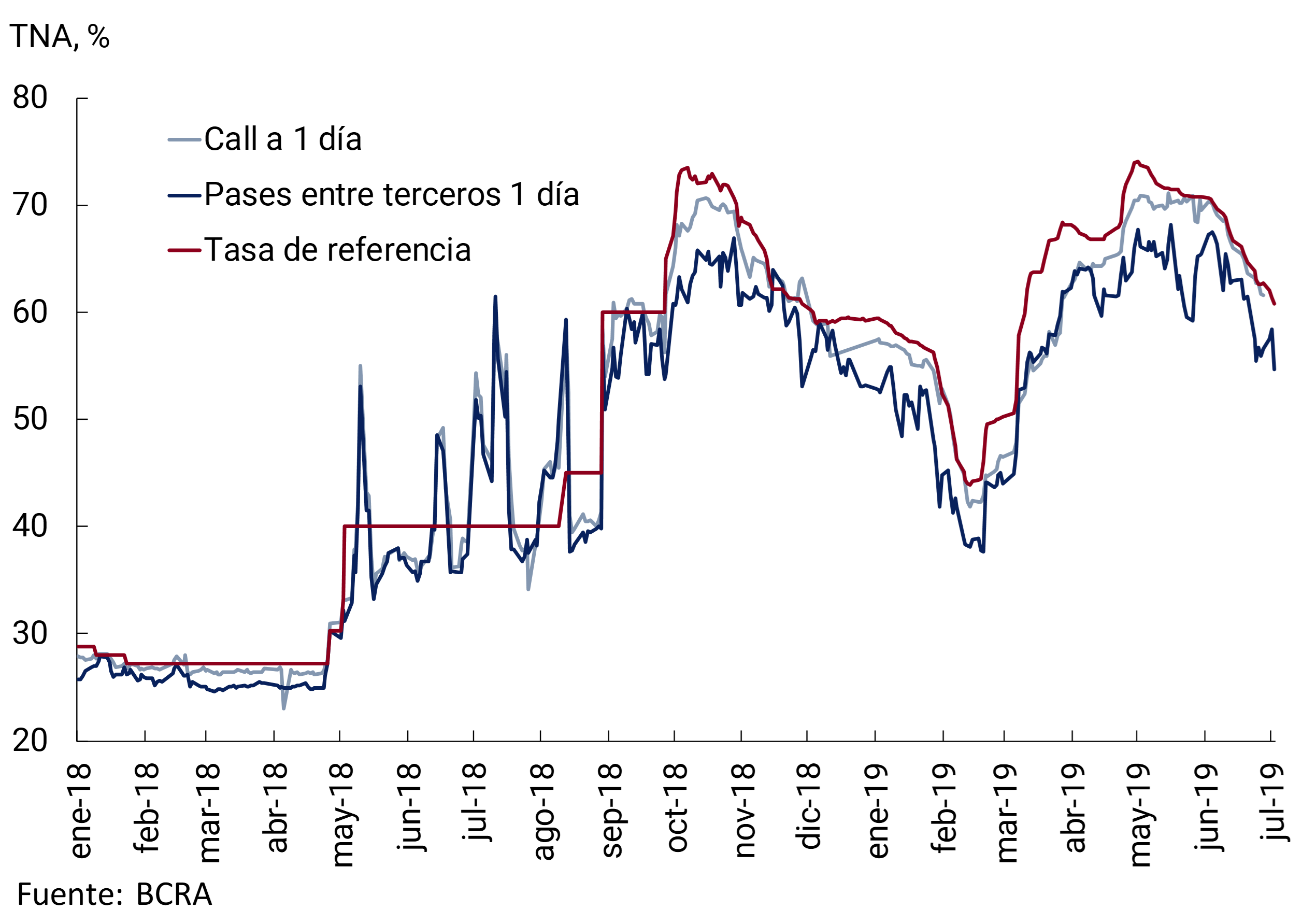
5.2.2 Private Sector Peso Deposits Held Steady During the Quarter with Tighter Rate Spreads
The main passive interest rates accompanied the rise in the reference rate during the month of April and then fell more moderately than the LELIQ rate in the months of May and June, which caused a reduction in the spreads of the passive rates in relation to the reference rate in that period.
During the quarter, the differential trajectory of the retail interest rate with respect to wholesale interest rates was highlighted. While the rate of fixed terms up to $100,000 remained stable during the months of May and June at around 46.7% annually, the BADLAR and the TM20 of private banks fell 5.9 p.p. and 6.4 p.p. in the same period, reaching levels of 47.5% and 48.6% annually, respectively (see Figure 5.14). This rapprochement between the retail rate and the wholesale TM20 and BADLAR occurred in the context of the measure taken by the Central Bank in which the possibility of making fixed-term deposits in pesos online without the need to be a customer was established (see Section 5).
Figure 5.14 | Main passive interest rates in the financial system
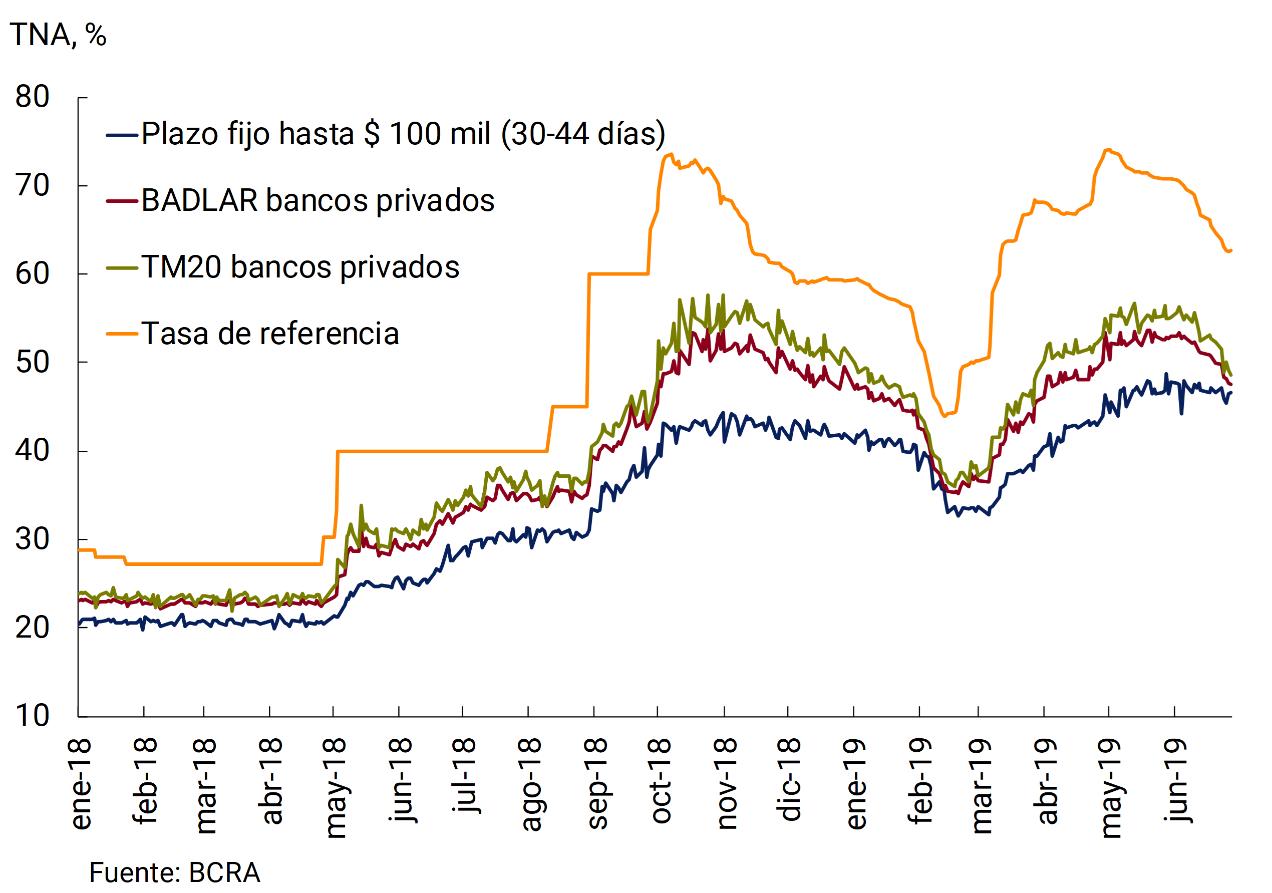
Private sector deposits in national currency increased at an average rate of 2.8% per month in nominal terms without seasonality during the second quarter of the year, led by the increase in demand deposits (+3.2% monthly average), while fixed-term deposits showed a 2.5% monthly increase. In real terms, this implied a contraction in total deposits of 0.4% per month on an average basis without seasonality during the quarter (see Figure 5.15).
Figure 5.15 | Private sector deposits in pesos (average monthly variation in the quarter – real without seasonality)
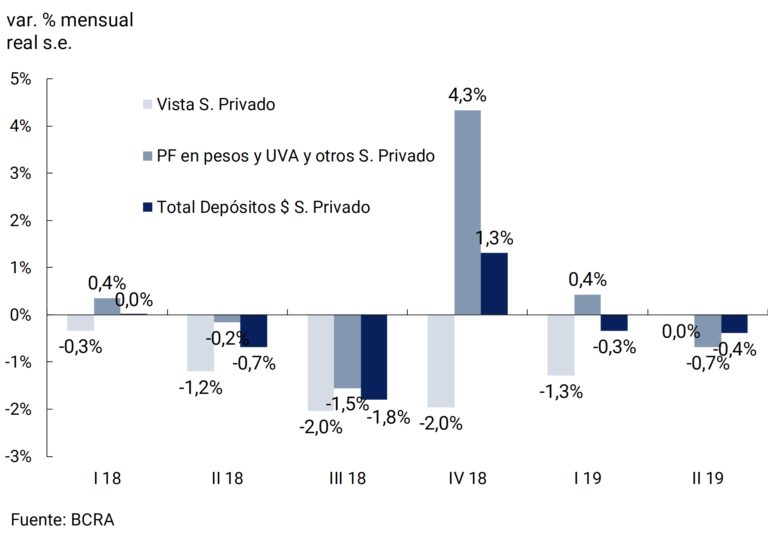
At the margin, time deposits exhibited a better performance in relation to demand deposits, growing by 4.2% monthly in June against 2.7% for the latter, thus reversing the behavior observed in previous months. This increase was mainly driven by deposits of human persons, whose growth rate was twice that of legal persons in the quarter (see Figure 5.16).
Figure 5.16 | Balance of fixed-term deposits in pesos of the private sector by holder
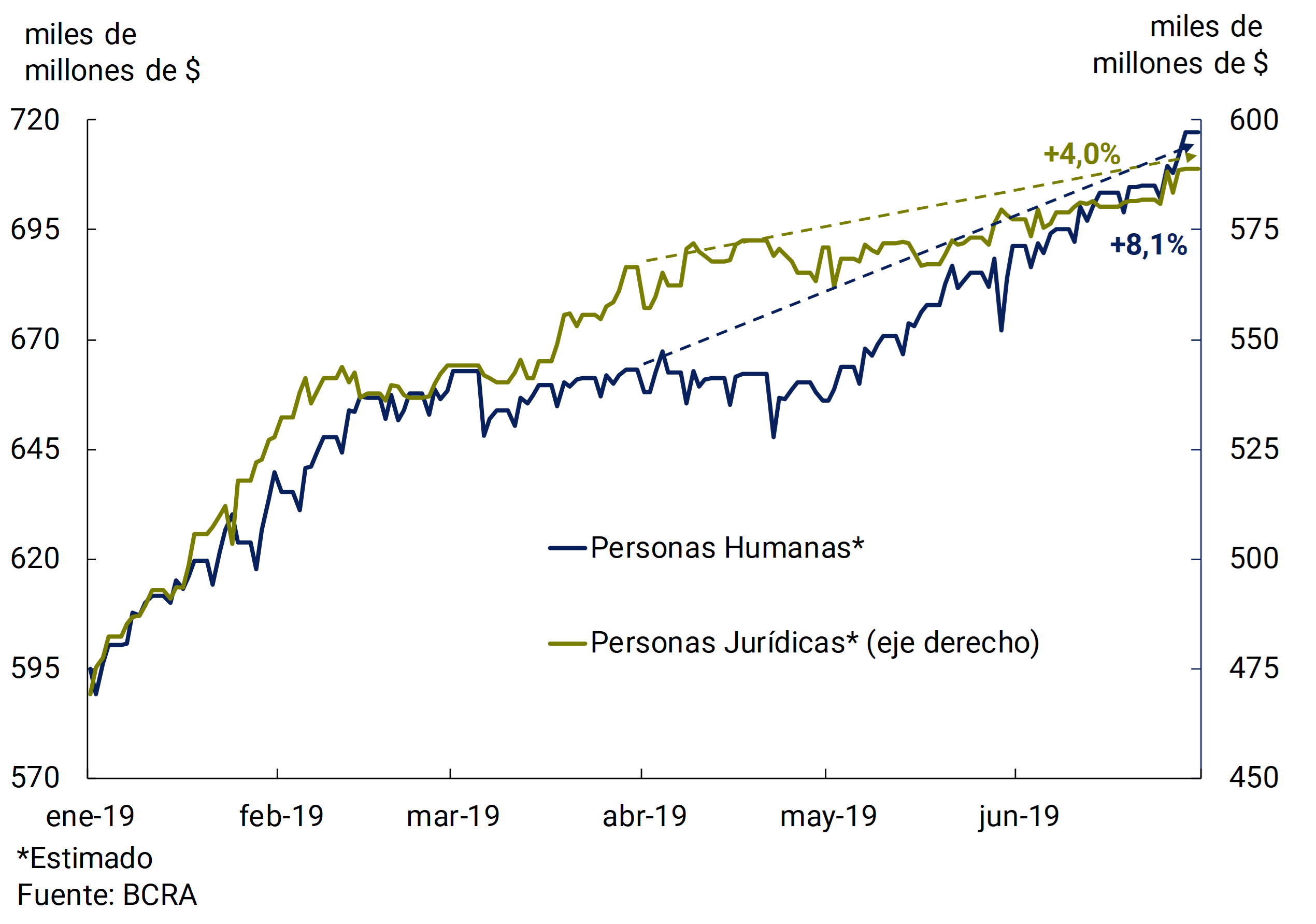
The share of UVA-adjustable fixed-term deposits in total private sector fixed-term deposits fell in June to 1.8%, from 2.5% in April. The fall in demand for these instruments was due to the combination of a reduction in monthly inflation, lower rates on these deposits (which fell 1.7 p.p. in the quarter to 4.35% per year on average in June) and higher nominal interest rates on non-adjustable fixed-term deposits (see Figure 5.17).
Figure 5.17 | Private sector fixed-term deposits adjustable by UVA (monthly average)
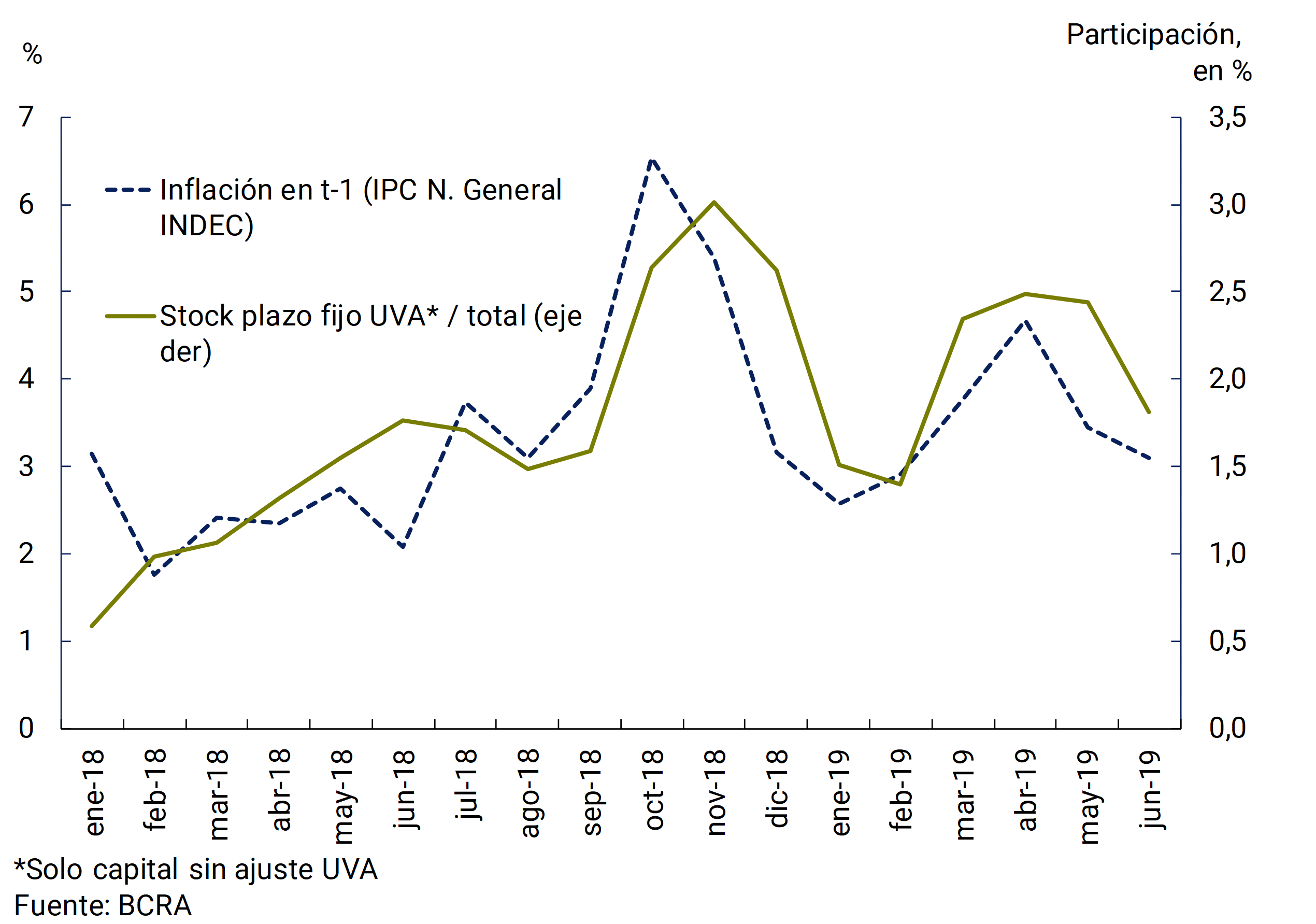
For their part, foreign currency deposits of the private sector maintained their growing trajectory during the second quarter, increasing 0.9% monthly average in foreign currency and thus reaching a new maximum of US$ 30,703 million on average in the month of June.
5.2.3 Bank credit to the private sector moderated its contractionary trend
Driven by the increase in the benchmark interest rate in April, rates on loans in pesos granted by the financial system also increased, which partially reversed as of mid-May in line with the movement of the reference rate (see Figure 5.18).
In the quarter, interest rates on signature and discount documents rose 2.5 p.p. and 5.6 p.p., reaching levels of 58.8% annually and 55.1% annually in June, respectively, while the current account advance rate, which is more closely correlated with the benchmark rate, fell 1.4 p.p. to 65.8% annually (see Figure 5.18).
The discount rate of documents, whose dynamics were affected during the period from March to mid-May of this year by the line of financing with preferential rates for SMEs launched by the Ministry of Production of the Nation, showed a strong increase from that date hand in hand with the exhaustion of the quota. thus reducing its spread with the reference rate.
The interest rate on personal loans increased in April and early May, driven by the rise in the reference rate, to levels of around 66% per year, remaining stable in the subsequent period despite the reduction in the LELIQ rate. For its part, the interest rate on pledge loans in pesos remained practically unchanged during the period, reaching an average level of 22.9% annually in June.
Figure 5.18. Main lending rates in the financial system

Interest rates on UVA-denominated loans were relatively stable in the quarter. Mortgage loans showed an increase of 0.2 p.p. compared to the average of the first quarter, reaching 6.1% annually on average during the second quarter, while those of pledges and personal loans fell 0.3 and 0.1 p.p. to levels of 14.9% and 18.7% annually, respectively.
Loans in pesos to the private sector moderated their rate of decline again compared to the previous quarter, with a contraction of 2.8% per month on average real without seasonality (see Figure 5.19), compared to the 3.7% monthly reduction in the first quarter. Unlike what was observed in previous quarters, loans associated with companies exhibited more moderate falls and in line with those that occurred in household consumer financing.
Figure 5.19. Loans to the private sector in pesos and dollars (average monthly variation in the quarter – real without seasonality and in original currency)
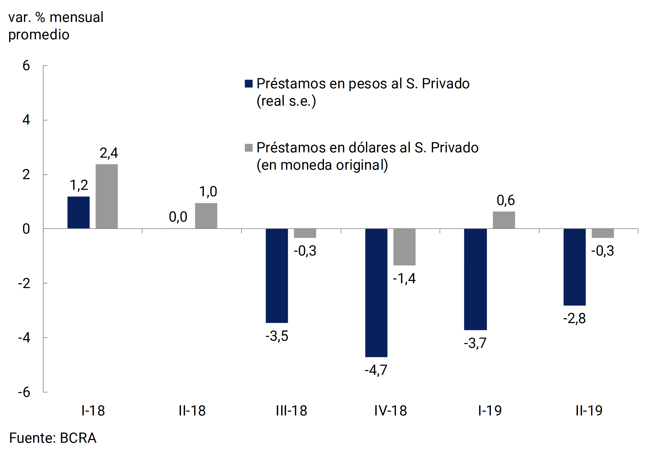
Foreign currency loans remained relatively stable during the second quarter, falling by an average of 0.3% monthly in original currency.
5.2.4 Financial institutions’ liquidity remained stable during the quarter
As a result of the relative better performance of deposits compared to bank loans in pesos, the ample liquidity of financial institutions (current account at the BCRA, cash, LELIQ, NOCOM, net passes and 2020 Bond) increased slightly in April and remained relatively stable during the months of May and June (See Chart 5.20). As a result, at the end of June it reached 63% of deposits, 1.5 p.p. higher than that recorded in March. This increase was explained by the greater holding of LELIQ (+3.3 p.p.), partially offset by the fall in current account balances at the BCRA (-1.4 p.p.). 47
Figure 5.20. Liquidity in pesos of financial institutions (in % of deposits in pesos)
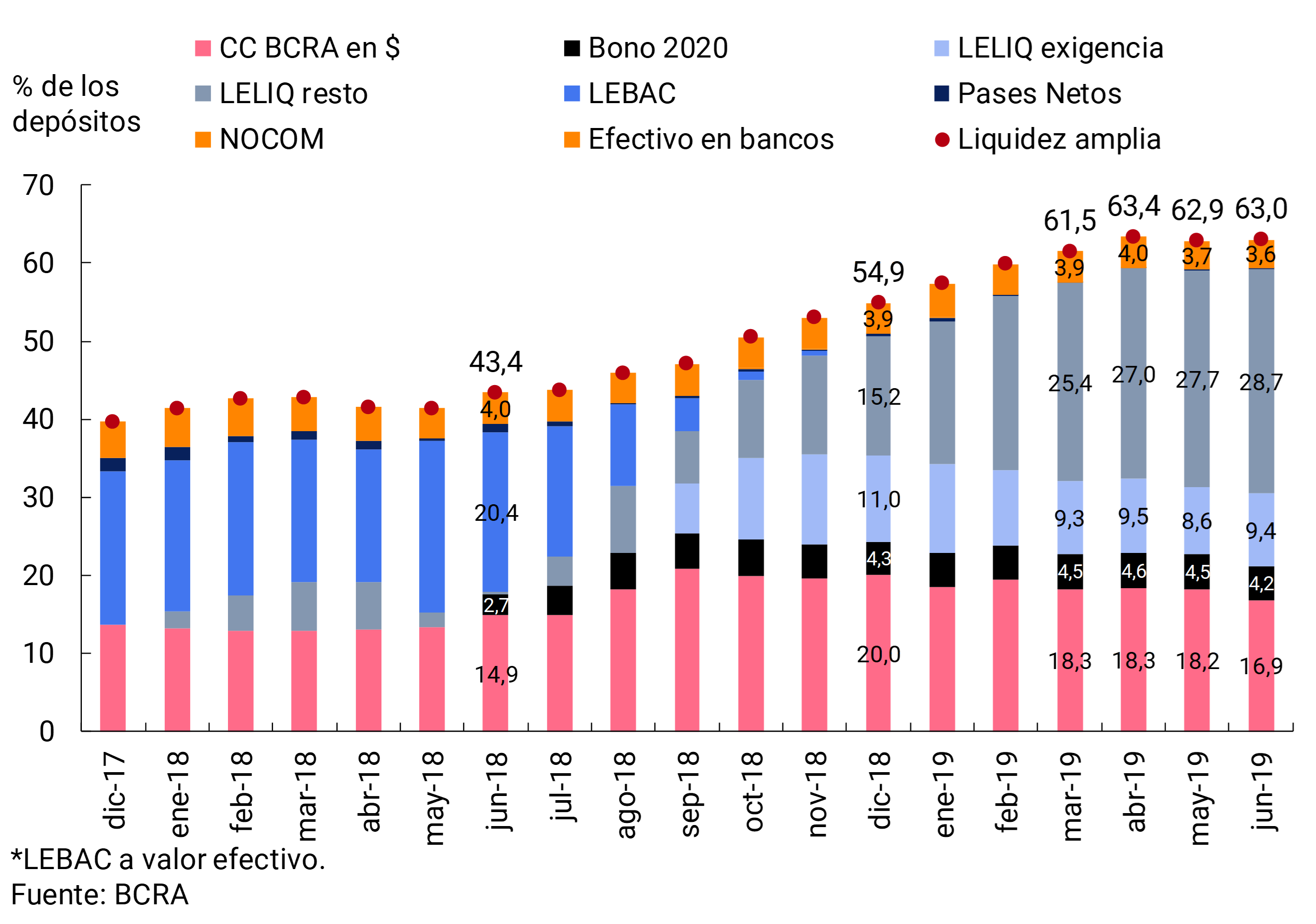
As of July, it was decided that the calculation of the minimum cash requirement in pesos will be determined on the average of the daily balances of the period prior to its integration (instead of the balances of the same period, as it was until then), as is the case in most countries of the world. with the aim of providing greater predictability to the financial system for liquidity management. 48 It was also decided that the calculation of minimum cash positions would be unified in the July-August and December-January two-month periods, and a reduction of 3 p.p. was established in the calculation of the minimum cash requirement as of July. 49
Section 1 / The US-China trade war
Trade between the United States and China grew steadily over the past three decades, exceeding $650 billion in 2018. The balance has always been in favour of the Asian giant (Graph 1), representing 48% of the total deficit in the exchange of goods of the world’s leading power. From the outset, the U.S. administration attributed this result to alleged improper trade practices by China. This was the justification for the United States to begin applying tariffs on a list of Chinese products in July 2018, which was expanded in the following months (Table 1). China responded in kind, giving rise to the most bellicose stage of the so-called “Trade War” between the two countries.
Graph 1 | U.S.-China Bilateral Trade
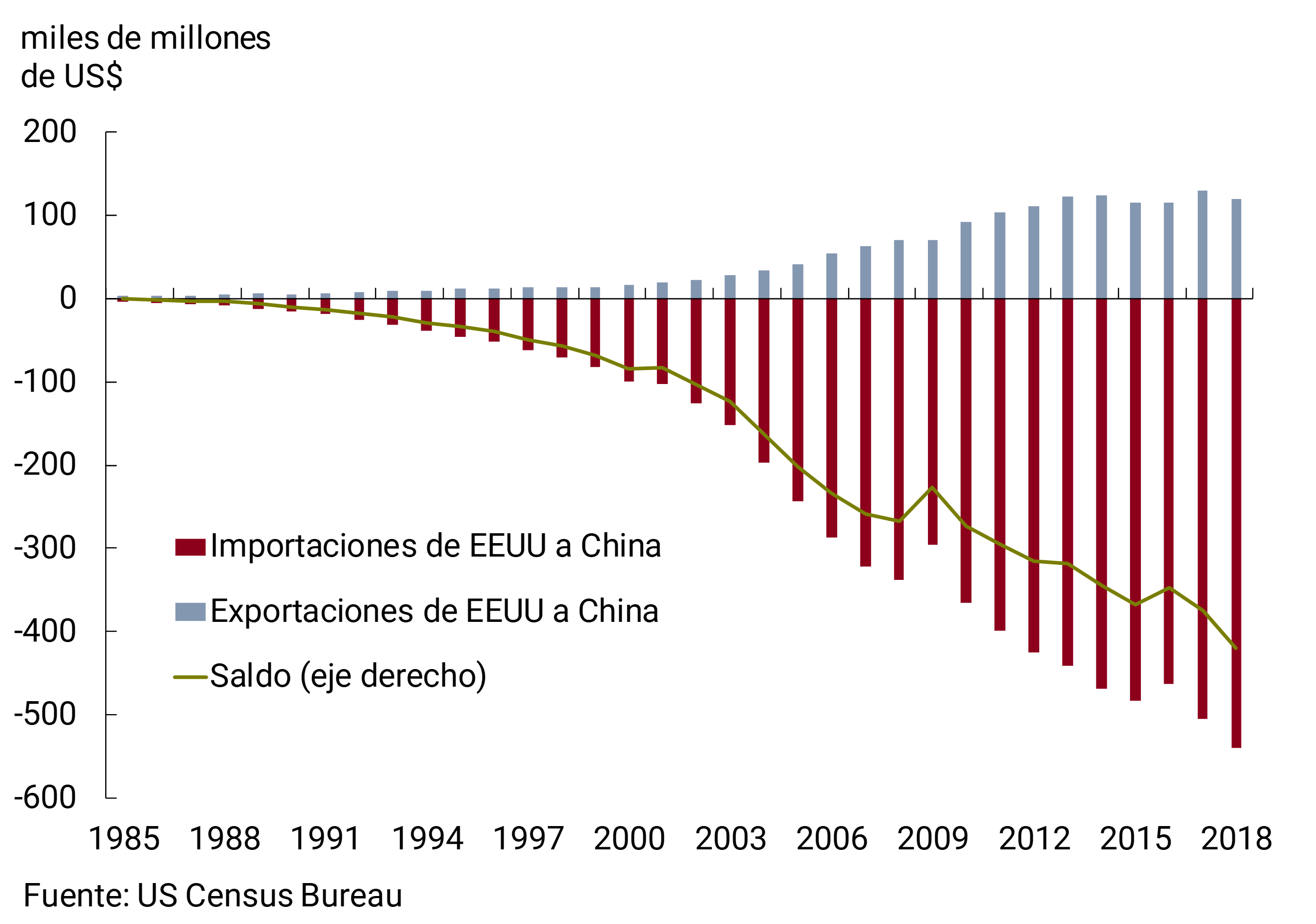
The products currently taxed by the United States accounted for about half of China’s imports ($250 billion) before the application of tariffs. The Chinese response has been more surgical. While tariffs were announced for products that accounted for some US$ 110 billion (about 80% of U.S. imports), only a portion of these products are taxed at the maximum tariff. Moreover, imports of hard-to-substitute goods such as aircraft and some types of machinery and intermediate goods remain tariff-free.
A first analysis of the impact of these measures suggests a fall in bilateral trade with negative effects on global trade. Since August of last year, there has been a sharp year-on-year drop in U.S. exports to China. Although imports took longer to respond, they started 2019 with sharp year-on-year declines, resulting in a reduction in the bilateral trade deficit (Graph 2). At the same time, although perhaps not the only cause, the growth in the volume of international trade is currently performing its worst since the international financial crisis. It should be noted that the growth of international trade is closely linked to investment and industrial production indicators, which have also been showing weakness (see the chapter on International Context). Given this, it’s no surprise that more than 600 U.S. companies recently signed a note to the U.S. president warning that a new round of tariffs would mean the loss of 2 million jobs and cut U.S. GDP by one percentage point.
Table 1 | Schedule of the application of tariffs

Graph 2 | Year-on-year changes in bilateral and global trade
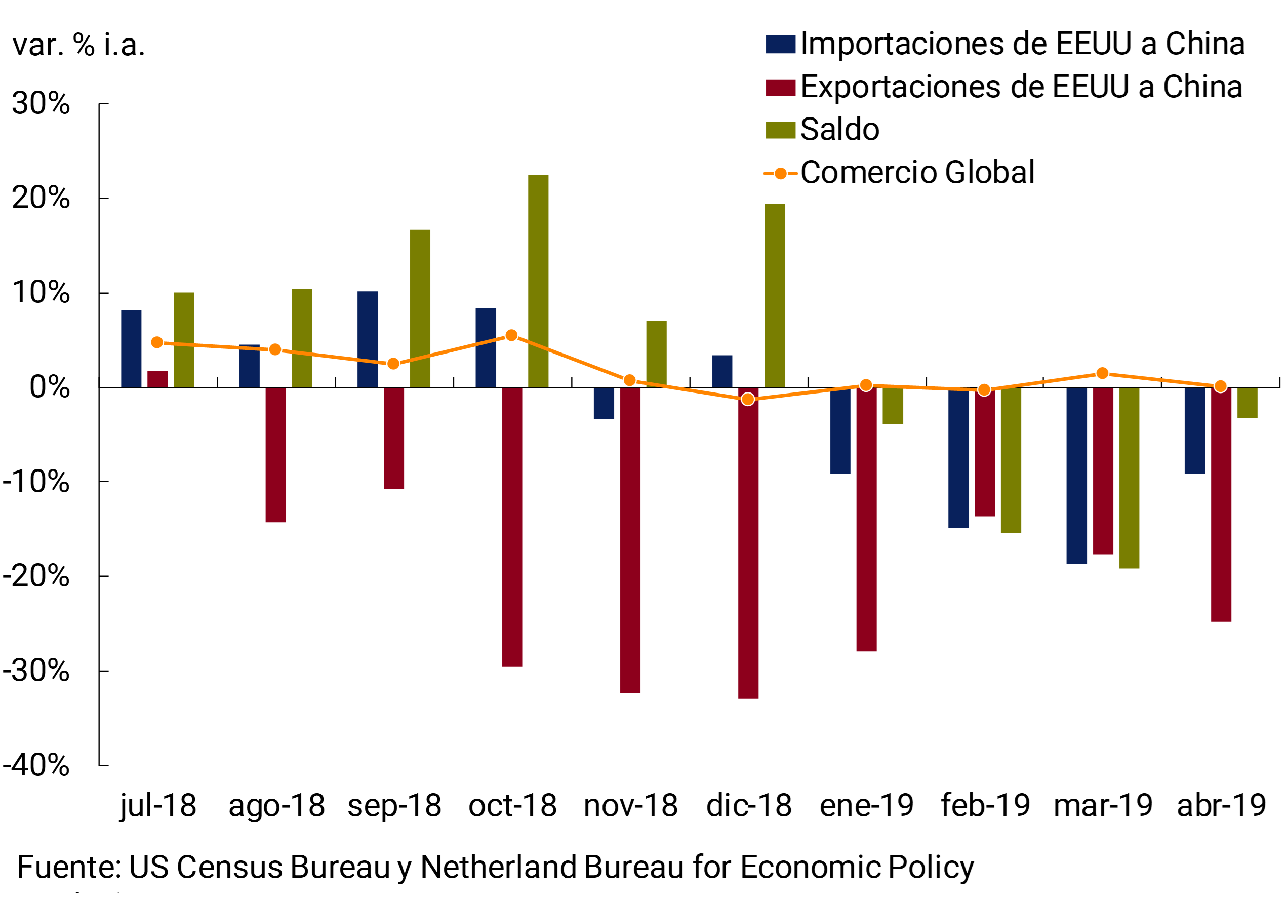
However, the result of the imposition of tariffs has resulted not only in a destruction of trade, but also in a certain reduction of the flows of goods to third countries. A recent report by the Council on Foreign Relations indicates that while U.S. exports to China of oil and industrial goods fell, this had no significant effect on either investment or production in these sectors, as supply could be sold in third countries. But the same was not true for soybeans, which account for about 10% of U.S. exports of goods to China. The imposition of tariffs on this oilseed caused the abrupt closure of the Chinese market for U.S. producers and a sharp drop in the domestic price compared to the international price, due to the impossibility of directing export flows to other markets. In effect, the U.S. government was forced to implement a subsidy to soybean producers to compensate for the negative shock suffered. China’s demand for soybeans was redirected to countries such as Brazil and Argentina, although the drought recorded during the last campaign prevented our country from taking full advantage of this situation.
When analyzing total exports from the United States by main items, the above is partially verified. Taking June 2018 as a reference point, prior to the entry into force of the tariffs, a fall in exports of raw materials, food and beverages is observed, although exports of automobiles also fell. The rest of the items have registered growth in the values exported (Graph 3).
Graph 3 | U.S. exports to the world (cumulative last 12 months)
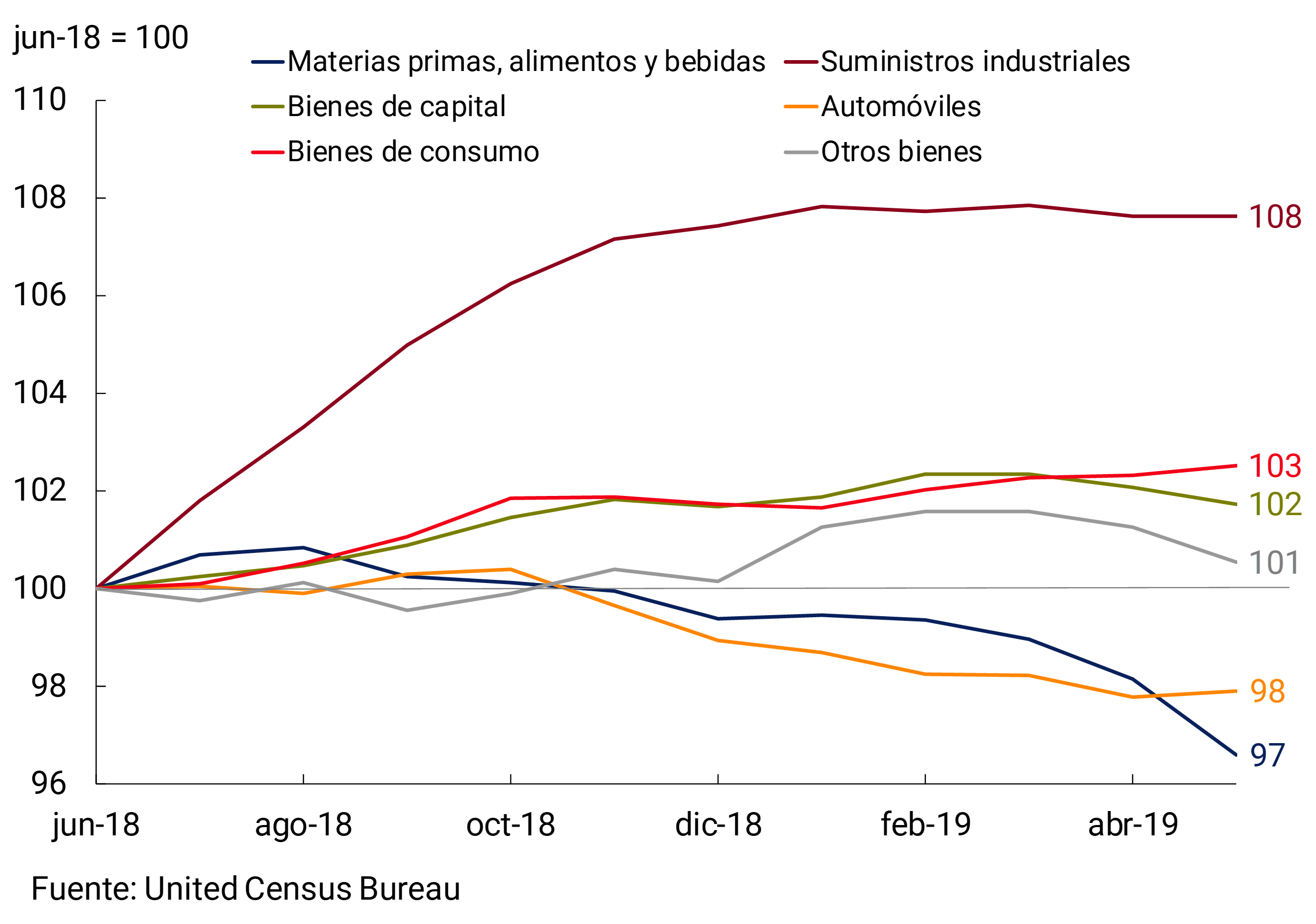
The diversion of China’s purchases to other countries was favored by the fact that, along with the imposition of tariffs on U.S. products, tariffs on countries producing the same goods were reduced. A report by the Peterson Institute for International Economics indicates that, for agricultural and seafood products, U.S. producers saw their average rates double, while for producers in other countries the rates were reduced between 2 and 3 percentage points.
The big question is whether these reconfigurations in global trade will last over time. Although at the recent G20 Leaders’ Summit held in Osaka, the US and Chinese presidents agreed to resume negotiations, there was no concrete progress and a new escalation cannot be ruled out. In this sense, it is convenient to review potential scenarios with different impacts on commodity-exporting countries such as Argentina.
First, there could be an agreement between the two powers that not only returns to the initial situation, but also includes quantitative targets aimed at correcting the bilateral trade imbalance. This hypothetical agreement could include, for example, that China increases purchases of soybeans and other commodities from the United States, reducing demand for other exporters, such as Brazil and Argentina, producing a trade diversion. In any case, the final impact of such an agreement is difficult to anticipate, depending on whether the United States increases its production of grains and oilseeds or simply stops supplying other markets to which the supply of South American countries could be redirected.
Another scenario to consider is that the commercial diversions that have been observed continue and become permanent. This can happen both in the event of a continuation of the trade war and in the case of an agreement that fails to restore trust between the two countries. In the latter case, both countries could aim to reduce mutual interdependence by diversifying their sources of imports, in order to reduce the impact of a new conflict. According to JP Morgan, part of the global production chains that currently supply the United States from China could move to countries such as Vietnam.
Some analysts recall that in 1973 the United States banned soybean exports to Japan for a week, enough for Japan to decide to start investing in expanding Brazil’s agrarian frontier, in order to reduce dependence on the United States. Will China follow a similar strategy? For its part, the United States is highly dependent on imports of rare earths50 from China, which do not represent a very significant amount, but are key for sensitive industries such as nuclear and military. Although there are other countries from which the United States could obtain its sources (Burundi and Malawi are mentioned as alternatives), putting the deposits of these minerals into production requires time and substantial investments.
An even more disruptive scenario was recently raised by former German Vice Chancellor Joschka Fischer, who argues that we are witnessing the beginning of a dispute for global hegemony that exceeds merely commercial issues. This can be seen both in the strengthening of nationalist discourses in both countries, as well as in the disputes over technological leadership (e.g. the Huawei case) and in the growing disagreement regarding the one-China policy (rumors of arms sales from the United States to Taiwan and support for the protests in Hong Kong). According to Fischer, after three decades of a single global market governed by the rules of the World Trade Organization, the world is once again heading towards the separation between two spheres of economic influence, where small countries may be forced to choose between one of them. Without a doubt, this is the worst scenario that the global economy and our country in particular could face.
Section 2 / Agricultural Harvest 2018/19
The 2018/19 Argentine agricultural season, which is being harvested, reached a record volume of 146 million tons of various grains and would directly contribute about 1.7 p.p. to the variation in GDP in 2019.
Likewise, and as a result of record production, the value of exports will expand in the coming months, contributing to improving the external and fiscal accounts. Net exports of the main agricultural products would increase in 2019 by about US$4,400 million compared to the previous year, implying an additional collection of export duties of US$1,300 million. Based on the first surveys of planting intentions, expectations for the 2019/20 Argentine campaign are auspicious and suggest – adopting historical assumptions – that production would return to around the highs reached recently.
Graph 1 | Argentine Agricultural Production
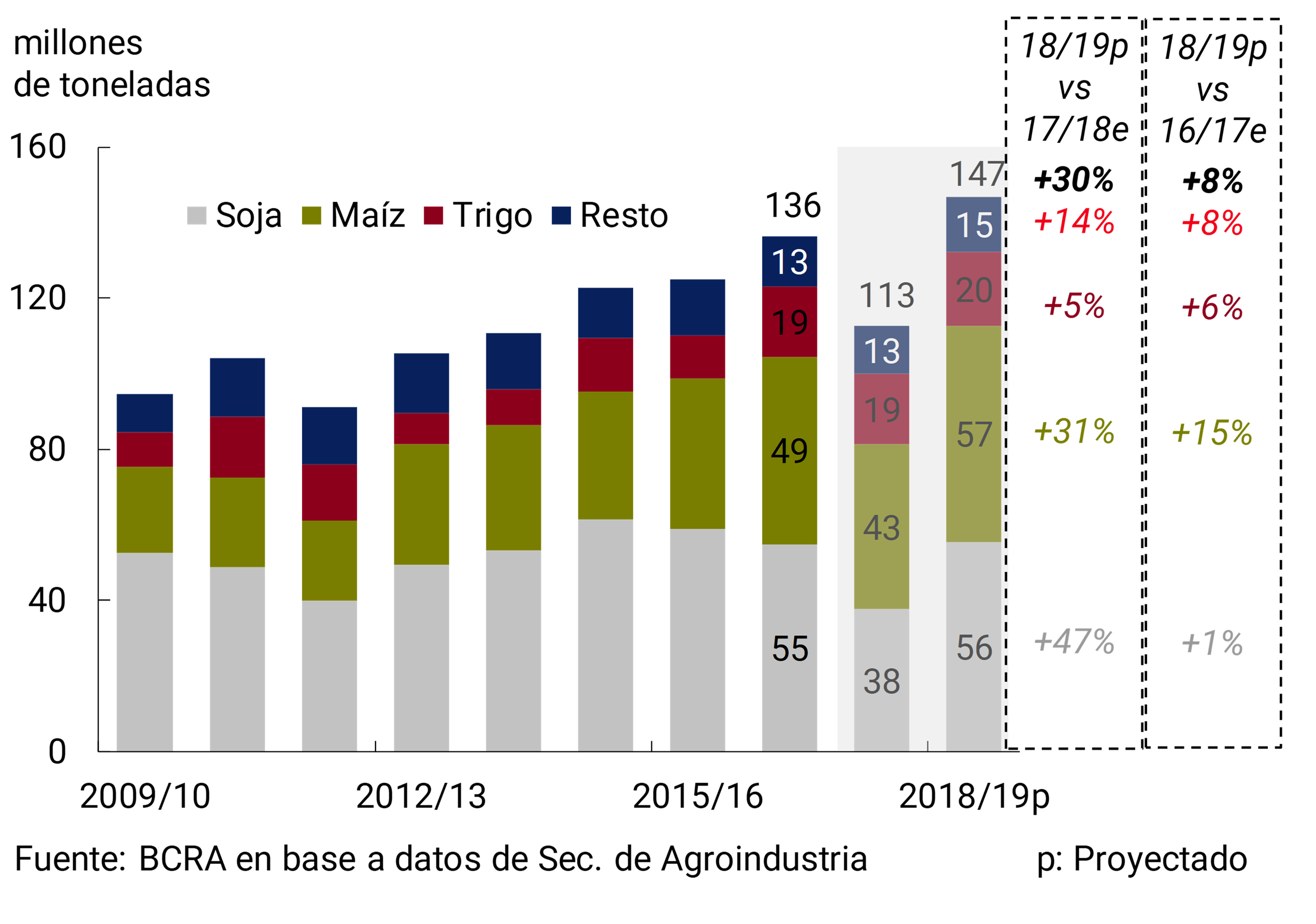
In the 2018/2019 agricultural campaign, the production of 57 million tons of corn stands out, which for the first time since 1997 – for a season without drought – exceeded soybean production. Thus, the weight of soybeans in the total harvest is at the lowest level for normal seasons since 2000, reflecting greater crop diversification. Total agricultural production increased by about 30% compared to the records of the previous season, which had been negatively affected by a major drought, and about 8% compared to the previous peak (see Graph 1).
After the severe drought in the previous agricultural season, the notable expansion of the 2018/19 harvest has a positive impact on economic activity this year (see Graph 2) and will drive other associated sectors.
Graph 2 | Agricultural production and value added of crop-producing sectors
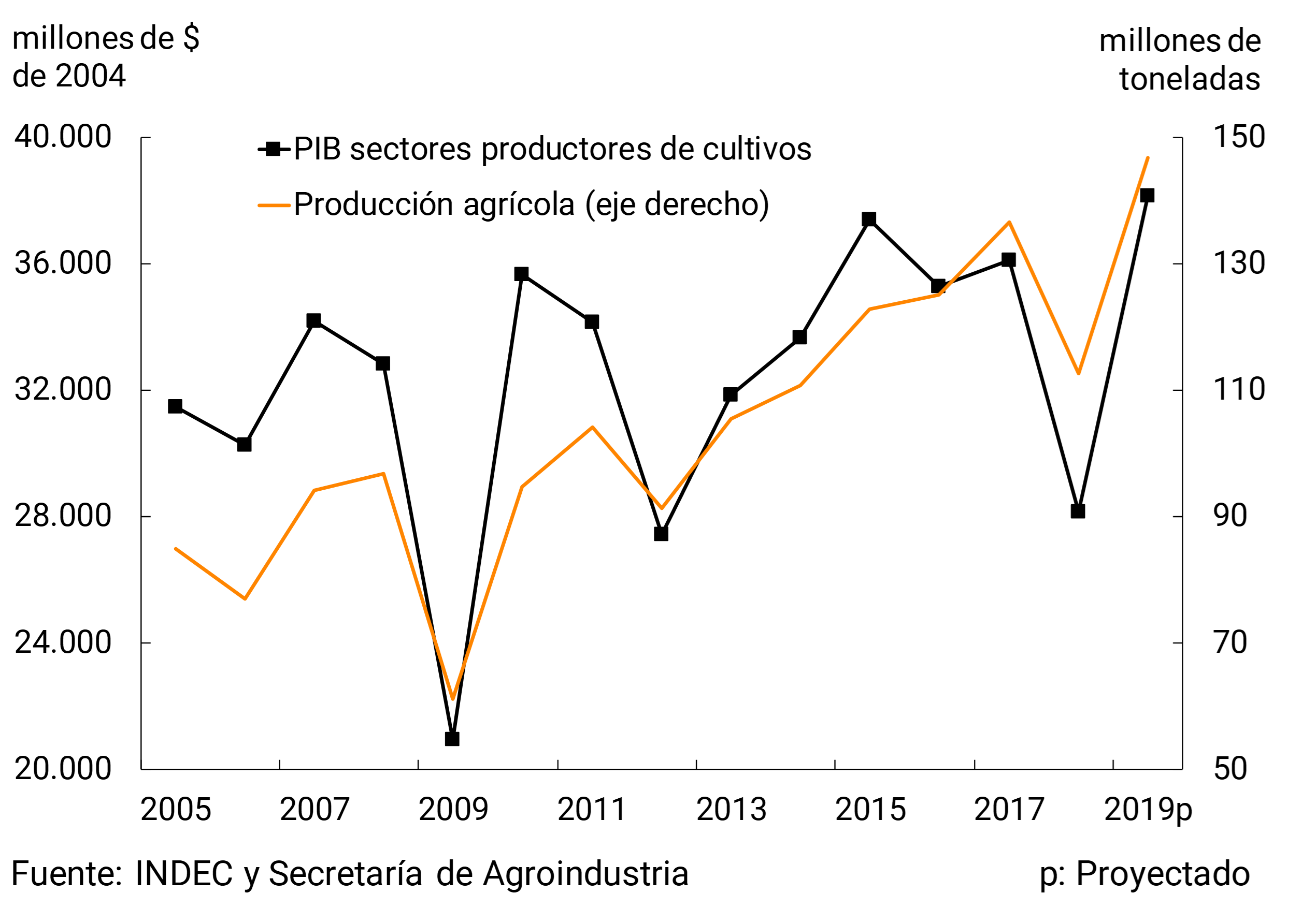
The marketing of the crop season of the coarse crop between April 2018 and March 2019 will continue in the coming months as producers sell their production. In the case of maize, cumulative purchases by the export sector have increased at a good pace, as has price fixing, in line with the expected significant increase in exports of this cereal (see Chart 3).
Graph 3 |Cumulative purchases of corn by the export sector
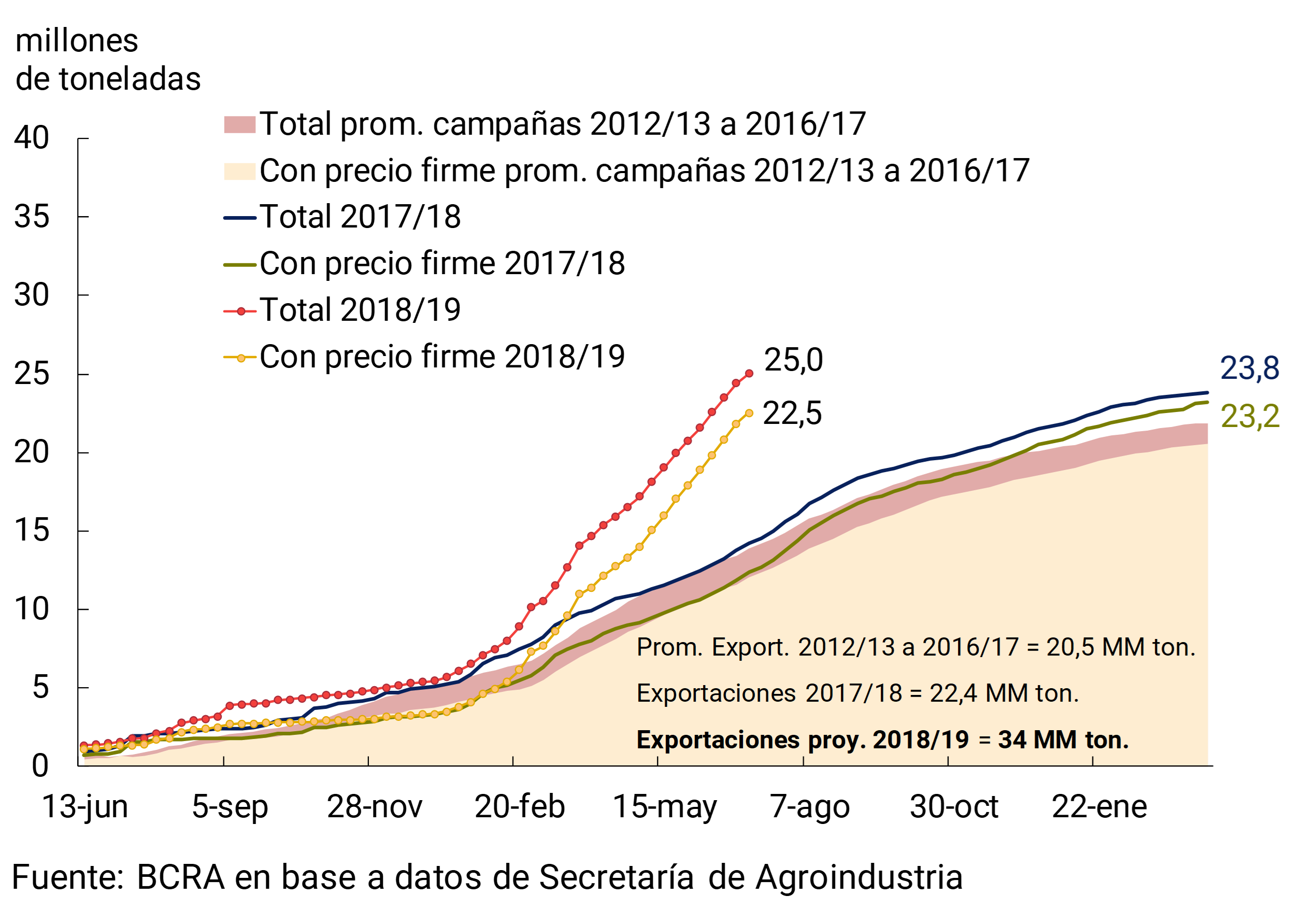
In the case of soybeans, cumulative purchases by the export sector and industry have increased at a rate similar to that of the average of the 2012/13 to 2016/17 seasons, with similar production volumes. It is expected that in the coming months the pace of price setting will increase, which has shown a certain lag so far this year with respect to the historical average indicated (see Graph 4).
Figure 4 | Cumulative purchases of soybeans by the export sector and industry
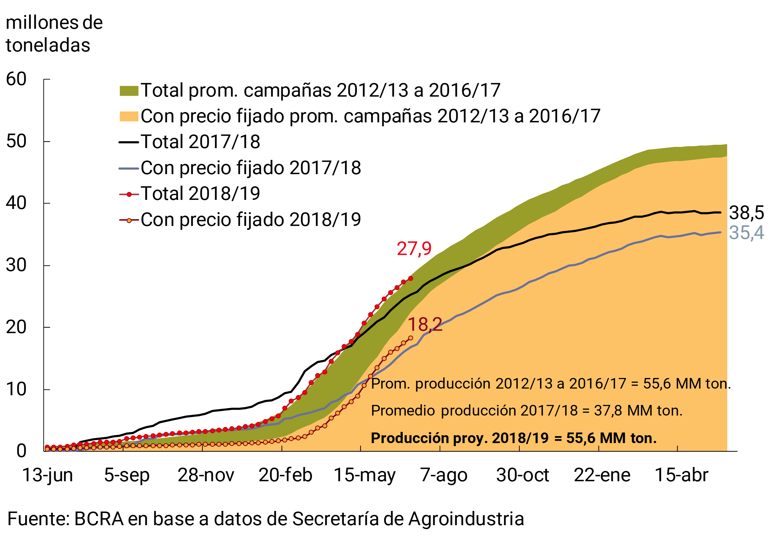
A boost in exports is expected in the coming months, particularly in net foreign sales of beans and soybean pellets and expellers (see Graph 5).
Graph 5 | Net exports of the Soybean Complex by Agricultural Cycle (Apr-Mar)
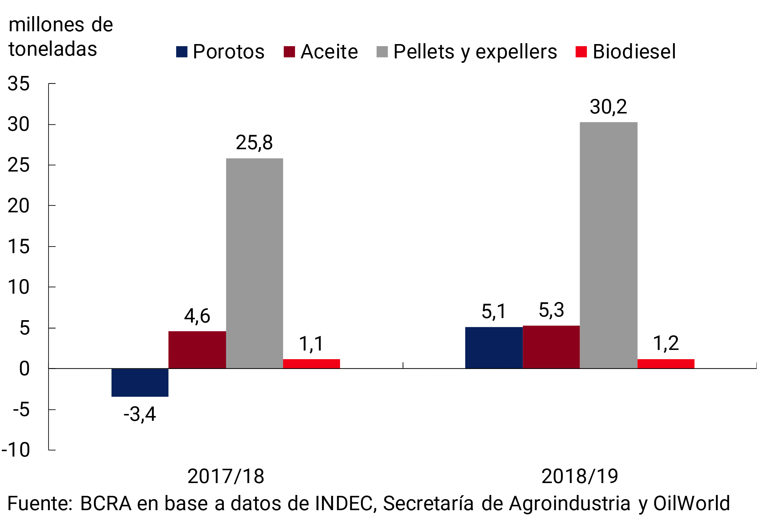
So far in 2019, the increase in the quantities exported (+24% YoY) did not translate proportionally into a rise in the values exported, which grew only 11% YoY. This is explained by the behavior recorded in the international prices of the main agricultural products exported by Argentina. In fact, international prices of soybeans and their derivatives fell compared to the average prices of 2018, due to various external factors such as the oversupply of soybeans, the “trade war” between the United States and China and the epidemic that afflicts pork production in China (African swine fever). These bearish factors were tempered by lower prospects for the soybean and corn harvest in the United States for the current season.
Section 3 / Nine months of operation of the monetary aggregate scheme
With the aim of recovering the nominal anchor after the episodes of financial volatility of 2018, in October of that year the Central Bank adopted a monetary policy scheme characterized by the strict control of monetary aggregates. 51 It consists of a zero growth target for the monetary base. 52 This is a concrete commitment, more directly linked to the tools under the control of the BCRA and easily verifiable by the public.
Initially, zero growth of the monetary base was established until June 2019 and the average balance of the monetary base of September 2018, of $1,271 billion, was taken as a reference, with seasonal adjustments in December 2018, June and December 2019. 53 Likewise, adjustments were foreseen for the interventions that the BCRA could carry out in the foreign exchange market, which were put into practice with the purchases of dollars in January and February 2019. 54
Inflation began to fall after the peak of 6.5% monthly in September last year, however, in February of this year it reversed to the upside. In addition to the inflationary inertia after the depreciation of 2018, the recomposition of regulated prices and the specific shocks to the meat sector were added. In this context, and to prevent these corrections from feeding back into inflation expectations, the COPOM decided to reinforce the contractionary bias of monetary policy. Thus, on March 14, 2019, it decided to extend the objective of zero growth of the monetary base until the end of 2019, eliminate the seasonal adjustment of June, and set as a new reference the balance of the monetary base of February 2019, of $1,343 billion, making permanent the overfulfillment of the target observed in that month (see Graph 1). 55 As of July, in view of the high seasonality of the demand for working capital as a result of the collection of Christmas bonuses and expenses associated with the winter recess, it was decided to reduce the minimum cash requirement on fixed-term deposits in pesos by 3 p.p. And in order not to relax monetary policy after this seasonal phenomenon, a reduction in the monetary base target was ordered from August to reach $ 1,298.2 billion in October, when this monetary effect would be fully compensated. 56
To keep the growth of the monetary base under control, the BCRA conducts daily auctions of 7-day Liquidity Bills (LELIQ) that can only be subscribed by banks. In this scheme, the Central Bank no longer sets a policy interest rate, but rather it is determined endogenously. It is the one that guarantees that the demand for LELIQ is consistent with the monetary base objective. This allows the interest rate to respond quickly to surprise changes in inflation, inflation expectations, or exchange rate expectations.
Graph 1 | Monetary base target
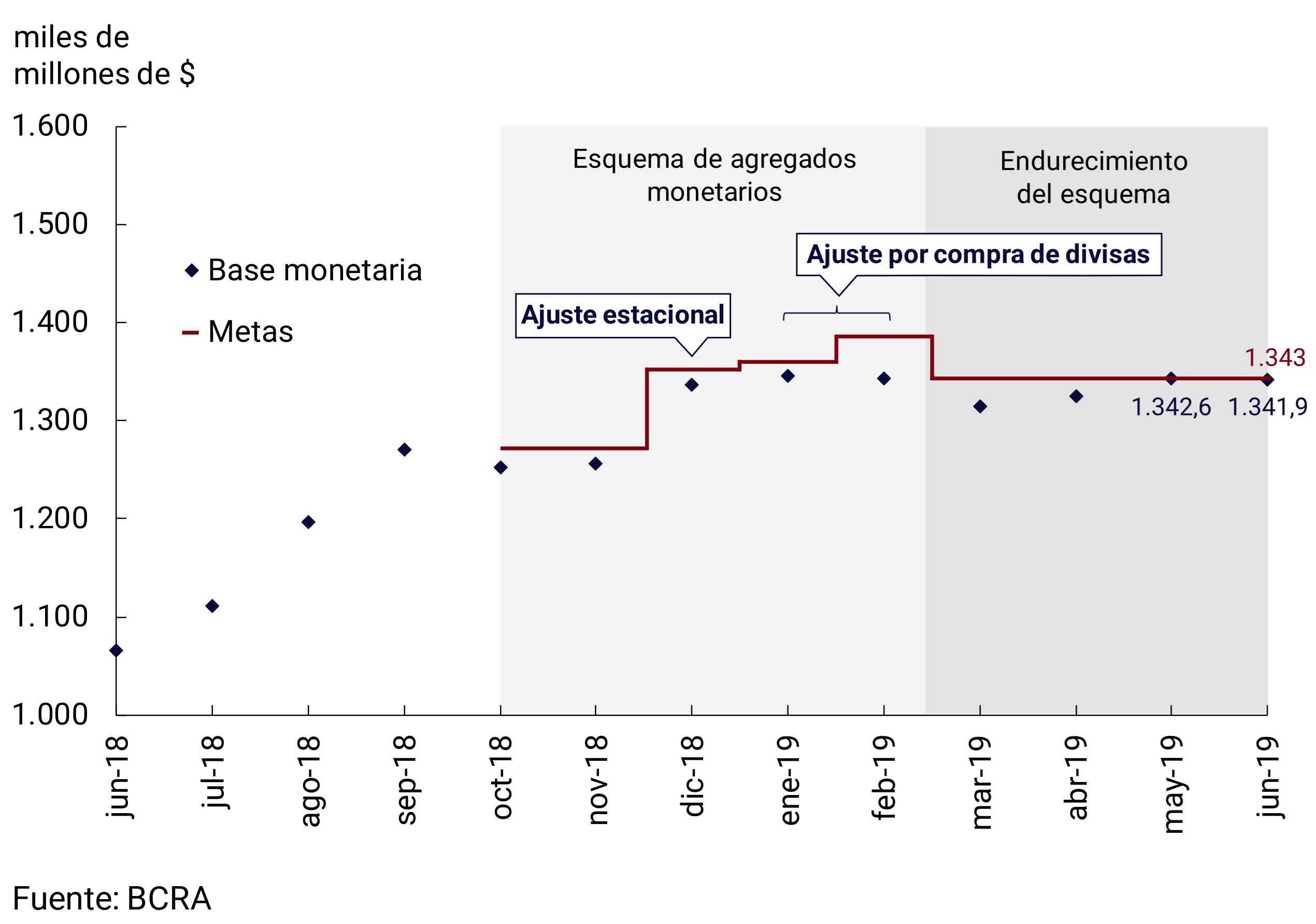
However, in order to prevent interest rates from being excessively volatile, the BCRA has the flexibility to manage liquidity conditions, adapting them to the intra-monthly seasonality of the components of the monetary base and to the transitory situations that may occur in the money market. In other words, zero growth in the monetary base allows the monetary base to grow on some days and fall on other days, while the variation in the average daily balances in the month is zero.
Given that the goal of zero growth of the monetary base is not a specific objective but a ceiling, the Central Bank also has the power to exceed it, as happened in the first months of the implementation of the scheme. This over-compliance prevents monetary conditions from easing (and interest rates from falling) in situations in which zero growth could be excessive, as is the case, for example, in those months when the demand for money is low seasonally or in the face of transitory shocks to the demand for money. In this sense, to ensure that monetary policy maintains its disinflationary character, a minimum interest rate was established, currently at 58% per year. 57 In other words, the BCRA undertakes to absorb the liquidity necessary to keep the interest rate from falling below that level, exceeding, if necessary, the goal of zero growth of the monetary base.
The monetary scheme is complemented by the definition of an exchange rate reference zone, the objective of which is to moderate episodes of excessive volatility in the exchange rate that could interfere with the disinflationary process, while preserving the benefits of exchange rate flexibility. The limits of the exchange rate reference zone do not constitute parities to which the Central Bank commits, but should be interpreted as guides on what can be expected from the BCRA’s behavior in each zone. If the exchange rate is above this exchange reference zone, the BCRA will hold daily auctions for the sale of dollars. These sales are not sterilized, which implies a direct retraction of the amount of money that contributes to stabilizing the money market. Similarly, if the exchange rate is below the exchange reference zone, the BCRA will hold daily auctions for the purchase of dollars.
Initially, the lower and upper limits of the exchange reference zone (which was called the non-intervention zone at the time) were set at $34 per dollar and $44 per dollar, and were adjusted daily at a rate of 3% per month until December 2018, 2% per month during the first three months of 2019, and 1.75% during the first fifteen days of April 2019. Given the persistence of exchange rate volatility, in order to reinforce the restrictive bias of monetary policy and avoid further shifts from the movement of the exchange rate to the inflation rate, it was decided to keep these limits constant until the end of the year at $39,755 and $51,448 (see Chart 2). 58 It was also established that, in situations of excessive volatility, the BCRA may intervene discretionally in the foreign exchange market, even if the exchange rate is located within the reference zone. 59 It was also decided not to hold auctions for foreign exchange purchases until July 2019 if the exchange rate was below the lower limit.
Graph 2 | Exchange rate and reference area
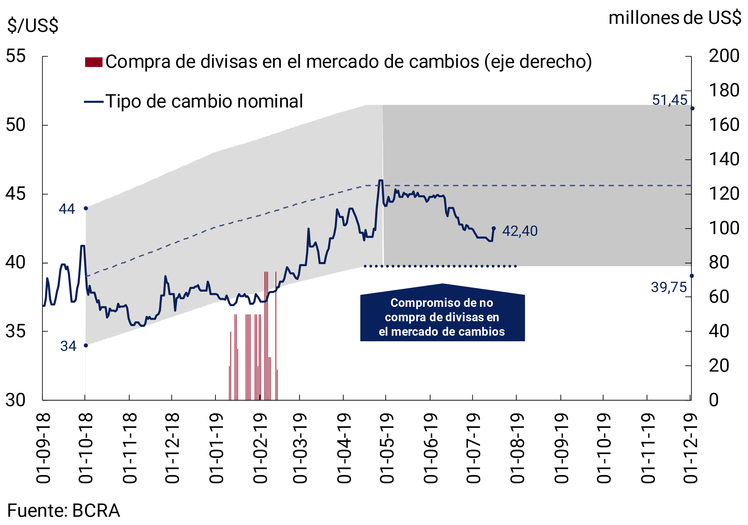
In summary, the monetary regime combines a strong nominal anchor, based on the control of the quantity of money, which has a relevant link with inflation in the medium and long term, together with the possibility of intervening in the exchange market to prevent situations of high volatility from affecting the disinflation process in the short term. Likewise, the BCRA introduced modifications to the scheme when the context required it, to strengthen it in the face of the emergence of new sources of nominal volatility. The latest changes introduced in March and April allowed inflation to resume a downward trajectory. However, disinflations tend to take time and are not linear, so the BCRA’s perseverance in its policy of strict control of the quantity of money is key to achieving a lasting reduction in inflation.
Section 4 / The goal of zero growth of the monetary base and the seasonal behavior of demand
Since October 2018, the BCRA implemented a new monetary regime with zero growth targets for the monetary base (WB). Given that the demand for the monetary base is markedly seasonal, it may be advisable to make adjustments to the targets and/or take measures to make the zero growth of the monetary base compatible with the seasonal oscillations (positive and negative) that this aggregate has. 60
To approach the concept of seasonality, it is useful to think that the economic series we observe (Y) are made up of three components that we do not observe directly: i) a trend-cycle component that reflects the medium/long-term evolution of the series (TC), ii) an irregular component or transitory shocks (I) and, finally, iii) the seasonal component (S). In the case of monetary aggregates, it is usually assumed that these components are combined in a multiplicative manner (Y = TC * I * S), which implies that seasonal oscillations change proportionally with the evolution of the trend in the series. If the trend increases, so do the seasonal effects and vice versa. 61
Graph 1 | Seasonal factors of the monetary base 2016-2018
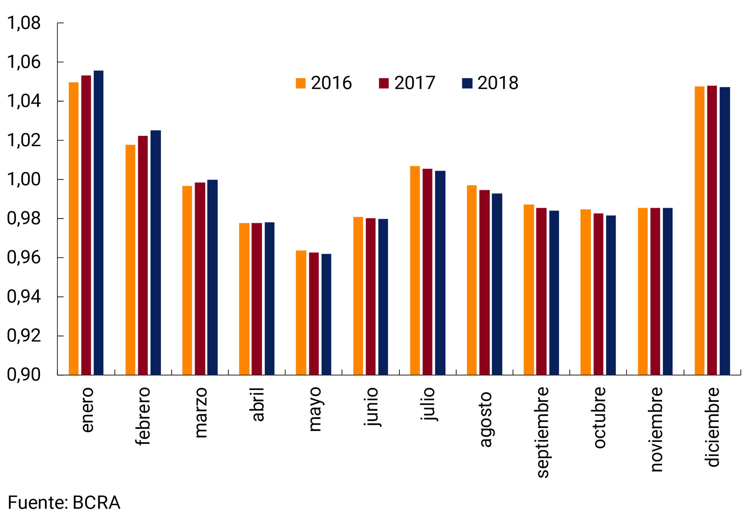
The seasonal component (S) includes the systematic events that occur within the year associated with climatic factors (e.g. harvest), institutional factors (e.g. payment of Christmas bonuses) and/or calendar factors (holidays, religious festivals, vacations, etc.). Like the seasons of the year, these events are repeated year after year with a regular periodicity that generates predictable and systematic fluctuations in the variables of interest. These fluctuations, relatively constant, are what is called seasonality and a series from which these systematic fluctuations are extracted is known as a seasonally adjusted or non-seasonalized series.
The unobservable nature of the three components mentioned requires some statistical procedure that allows them to be estimated from the observed data. To do this, the BCRA uses the X-13ARIMA-SEATS program, which basically uses a process of filtering by moving averages on the observed data and their successive transformations, which returns as a final product an estimate of each of the components indicated. 62
The estimation of the seasonal pattern allows us to obtain the seasonal factors of the BM, which indicate the direction in which seasonality operates in a particular month: a factor of 1 is indicative of a “neutral” month in terms of seasonality, while factors above (below) 1 indicate that there will be greater (lower) demand for BM with respect to a “neutral” month. Graph 1 shows the seasonality factors of the WB for the period 2016-2018. 63
Graph 2 | Monetary base: original series and without seasonality (in $ millions)
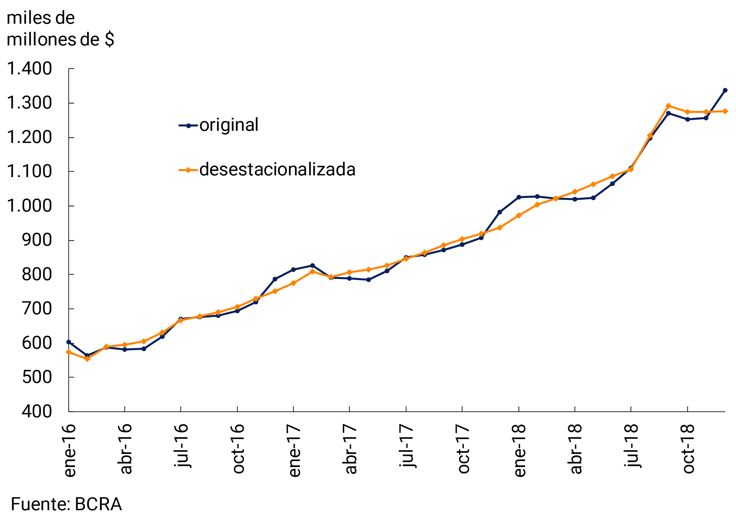
The estimation of seasonal factors also allows us to obtain the BM series without seasonality. To do this, the original BM data for each month are divided by the corresponding factor (S) to obtain the seasonally adjusted series (BM / S = BMSE = TC * I). 64 When it comes to a month with a seasonal factor above 1 (e.g. December), the seasonally adjusted series is lower than the non-seasonally adjusted series, and vice versa (see Graph 2). A series without seasonality, then, captures the movements of the trend-cycle (TC) and the impact of transitory shocks (I).
In addition, based on seasonal factors, the monthly contributions of seasonal behavior to the variation of the monetary base can be calculated. Figure 3 shows the monthly changes in seasonal factors for all months from 2016 to 2018. The months that contribute on average to positive seasonal growth are January, June, July and December. In these months, the demand for BM increases on average 0.5%, 1.8%, 2.6% and 6.3%, respectively, due to seasonal factors, explained by the payment of the Christmas bonus, the end-of-year holidays and the winter and summer vacations.
Graph 3 | Monthly contribution for seasonality 2016-2018 (in p.p.).
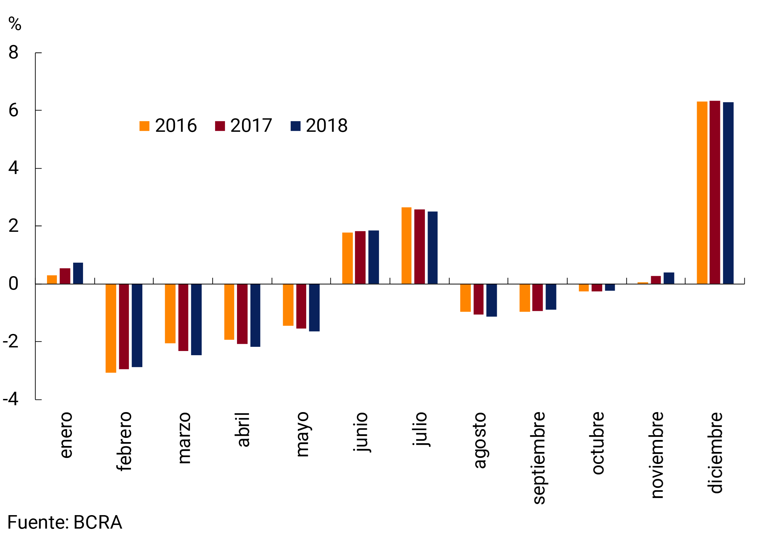
In the context of the current zero growth scheme of the monetary base, compliance with the target becomes more demanding in the months of high seasonality and less restrictive in the months of low seasonality. Therefore, the target for December, the month with the highest seasonal contribution of the year, foresees a seasonal adjustment of 6.3%. In the case of months with low seasonality, the Central Bank has the power to exceed the target, as happened in February of this year.
The BCRA also provided bimonthly minimum cash positions for the months of July-August and December-January, to make the months of high seasonality compatible with the monetary base target. It also decided to reduce the reserve requirements of fixed-term deposits by 3 p.p. as of July, to compensate for the seasonal rise in working capital demand. In order to maintain the contractionary bias of monetary policy, once this seasonal phenomenon has been overcome, the monetary base target will be reduced as of August. 65
Section 5 / Effects of the new online fixed-term operation for non-customers
As of April 30 of this year, the Central Bank established that bank users can make fixed-term deposits in pesos online at a financial institution without having to be customers of the same or carry out additional procedures. 66 These fixed terms are non-transferable and, once the period stipulated for the placement has expired, the principal and interest return to the original account. This operation does not imply additional costs for depositors.
To generate greater transparency and so that the user can choose in a simple way, the Central Bank made available on its website, a comparative table with the interest rates offered to customers and non-customers. This table is made up of the ten banks with the highest volume of deposits, of which four publish interest rates for non-customers, and nineteen other entities that also enabled this operation and began to report the interest rate for non-customers. 67 In this way, users can compare the interest rates offered by different banks and choose the option that is most convenient for them.
In the first two months of this operation, some 88,500 online fixed-term transactions were carried out for an approximate amount of $17,400 million. In May, some 37,900 operations were registered for an amount of $7,000 million, while in June some 50,600 operations were carried out for $10,400 million, which implied a monthly growth of 33.5% of the amounts and 50.4% of the amount placed. 68 The average amount of the placements was close to $200,000, which shows that it was concentrated in the segment of retail depositors. In this sense, this new operation contributed to the growth observed in the fixed terms of families from May (see Figure 5.16). The interest rates agreed in May and June were between 46% and 57% per year, with a weighted average of 55% per year, a level significantly higher than the average interest rates of retail operations in that period (around 47% per year).
This is a novel operation and its full effect will be known over time as it continues to gain participation among savers. However, two months after its implementation, fixed terms for non-customers have already had an appreciable impact on competition in the retail segment. The interest rate differential between wholesale and retail fixed-term interest fell significantly between early April and mid-July (see Chart 1). The spreads between the BADLAR rate and the TM20 rate of private banks with respect to the rate of fixed terms of less than $ 100,000 fell 4 p.p. and 6 p.p., respectively. 69 The spread between the reference rate (LELIQ) and the retail rate was also reduced by about 9 p.p. in the same period. The reduction in the retail spread explains why the interest rate for small deposits has remained stable as of June, while the wholesale rates, BADLAR and TM20, fell by 5 p.p. following the evolution of the LELIQ rate (see Chart 2).
Graph 1 | Wholesale vs. retail interest rate spread (in p.p.)
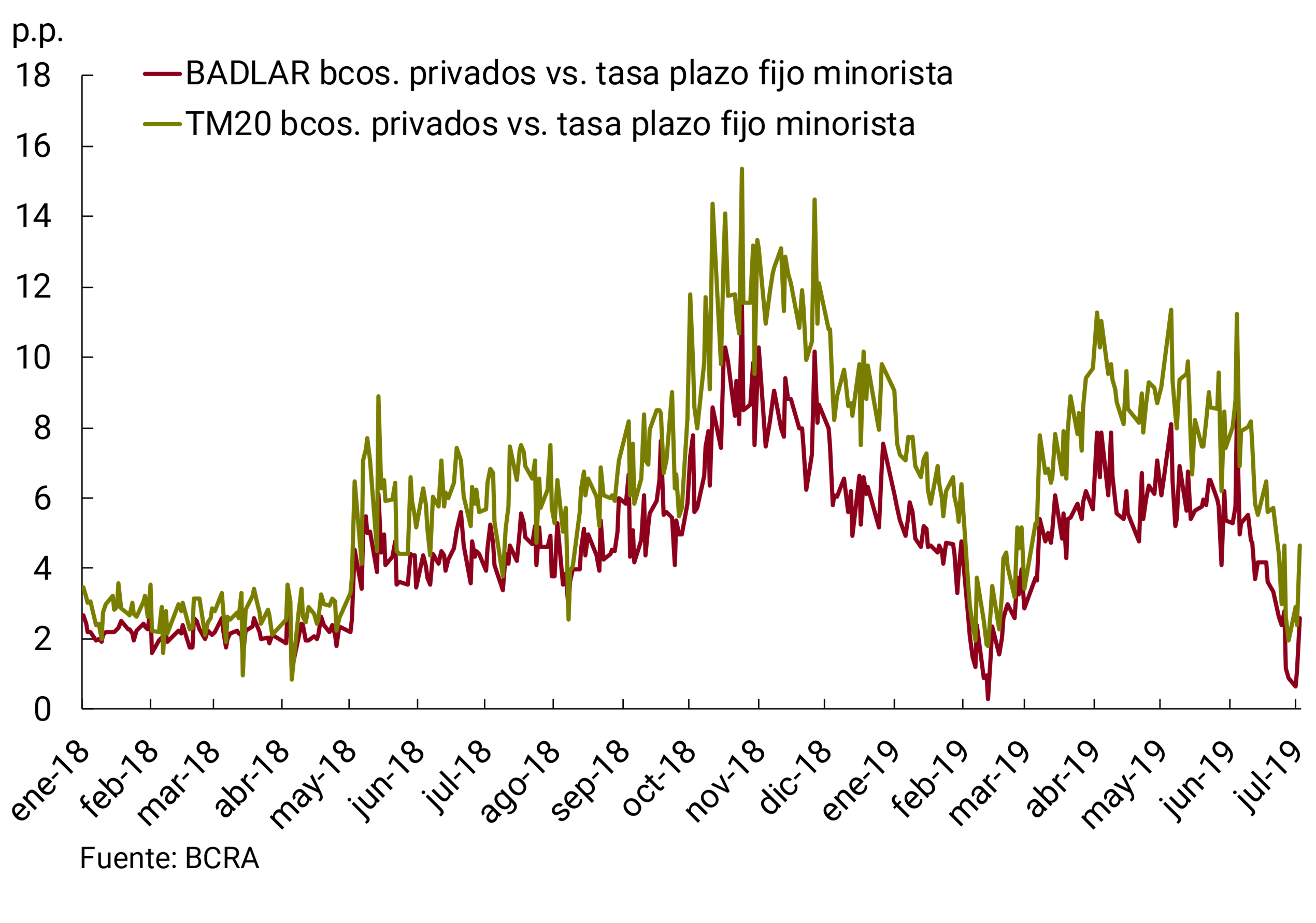
This new operation stimulates competition among financial institutions for retail depositors and strengthens the mechanism for transmitting the interest rate of the LELIQ to the rest of the interest rates in the economy. This results in higher returns for savers and collaborates with the objective of generating positive real interest rates, which are necessary to encourage savings in pesos and achieve a sustained expansion and expansion of bank credit.
Graph 2 | Wholesale and retail passive interest rates
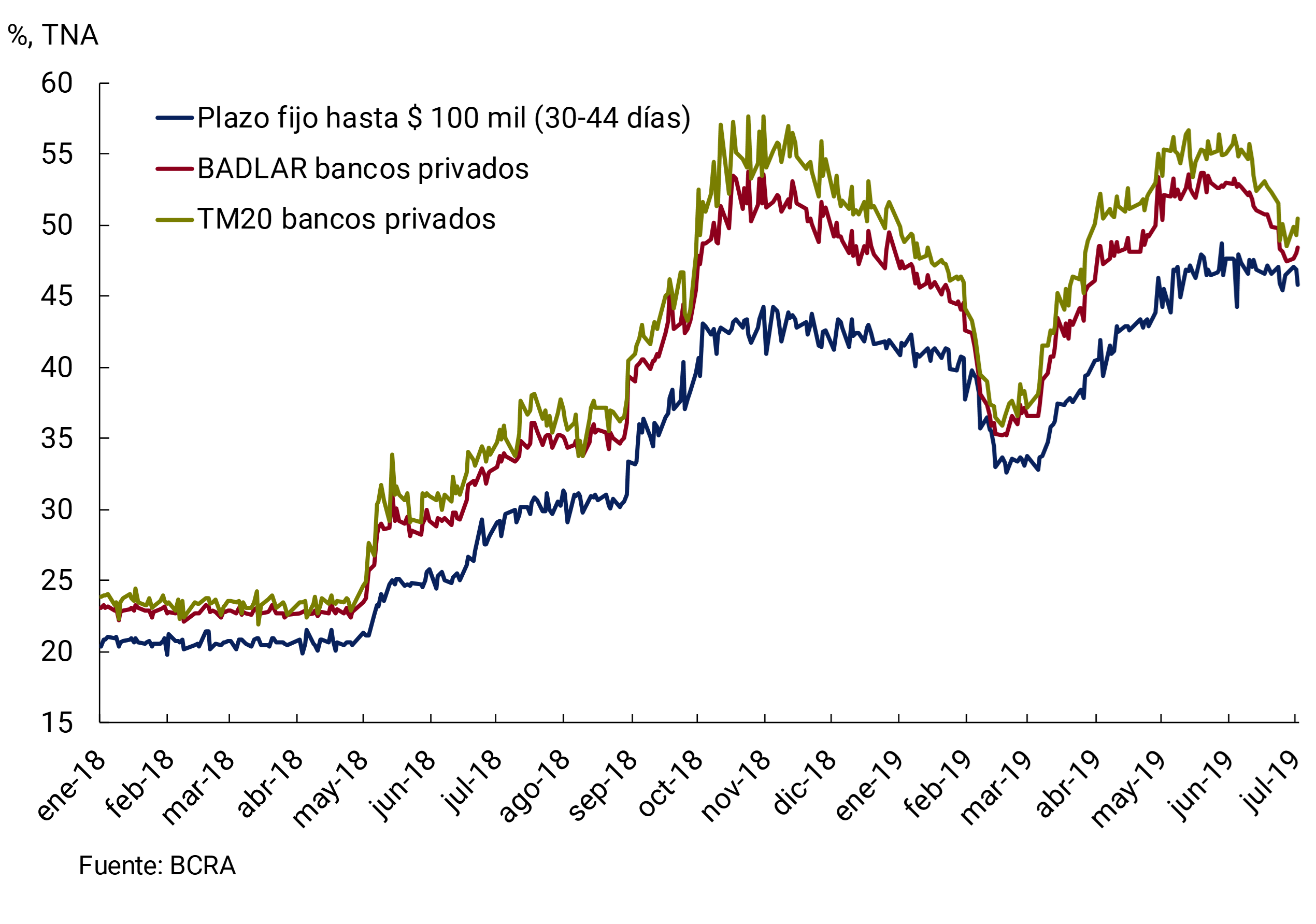
1 The world economy, which had been characterized during 2017 by relatively synchronous growth at the global level (4% YoY), began to show some partial slowdown during 2018 (it grew 3.8% YoY in the first half of the year and 3.2% YoY in the second), and seems to be going towards a lower generalized dynamism in 2019. However, some recently released one-off activity data would indicate some improvement in the margin, but it is still too early to know if they correspond to a change in trend.
2 It is defined as the interest rate at which it becomes profitable for a financial institution to exchange current account deposits at the central bank for cash. The recent experience of many developed countries with their unconventional monetary policies is that the elb is not zero, but negative, due to the cost of hoarding cash. This is why in the current literature they refer to the elb, instead of the zero lower bound. De Fiore & Tristani, 2018. ECB WP N° 2018. (Un)conventional policy and the effective lower bound.
3 For more details on what WLTPs are, see this link.
4 Close to the publication of the IPOM, it was known that the GDP growth rate in year-on-year terms slowed down again in the second quarter of 2019 to 6.2%.
5 According to the Commodity Price Index (CPI) published daily by the BCRA, which reflects the evolution of Argentina’s main export commodities.
6 To evaluate the intensity of activity growth, the seasonally adjusted monthly variations of 51 indicators (see IPOM April 2019) corresponding to the month of May were calculated. Each variation was subtracted from the average observed since 2004 and divided by its historical volatility. The standardized or normalized variations are presented in order from lowest to highest in the “heatmap” type graph, where the intensity of the green (red) color defines a more marked growth (fall).
7 INDEC measures Gross Fixed Capital Formation (GFCF) as the total value of fixed asset acquisitions that are used in production for more than one year. The FBCF is composed of durable production equipment and construction.
8 Part of this increase is explained by the increase in the rate of VAT collections DGA (General Resolution 4461/2019).
9 The ANSeS has budgeted to disburse up to $124,000 million, as of June 25, the ANSeS had granted $55,367 million.
10 Between January 2016 and April 2019, the program had a turnover of approximately $352,000 million in a total of 114 million operations. Currently, 262,803 businesses throughout the country are adhered to.
11 The mortgage loan is granted by one of the participating banks (Banco Nación, Banco Provincia or Banco Ciudad) and the National State provides a subsidy of up to 18,000 UVAs ($674,000). The payment term is up to 30 years for homes with a maximum value of 140,000 UVAs.
12 The programme was extended to July 2019 and was called Julio Okm.
13 Up to $750.00 the final discount will be $50,000 per unit. From that amount, and up to approximately $2 million – the final limit on which the internal tax or luxury tax begins to be paid – the bonus will be $90,000. The discount is for the purchase of 0 km cars in cash or financed, but not for those acquired through savings plans.
14 The estimate of activity is based on the evolution of the Synthetic Indicator of Construction Activity (ISAC) and the number of employed people in the sector in the SIPA-AFIP. These indicators are used to extrapolate the sectoral Value Added in a weighted manner according to the shares of the surplus and the remuneration to employees and mixed income, respectively.
15 http://www.construar.com.ar/2019/04/construar-informe-de-la-obra-publica-marzo-2019/.
16 The methodology for estimating the teaching and health services is linked to the staffing dedicated to these tasks and that is why the series show since the base year (2004) a positive long-term trend that accompanies the natural growth and the increase in the coverage of these services.
17 Between the first quarter of 2016 and the same period in 2019, the value added by the public administration sector grew at an average rate of 0.4% y.o.y., a rate much lower than the 3.2% y.o.y. recorded between 2007 and 2015.
18 The Industrial Production Indicators (IPI) of INDEC, the consulting firm Orlando J. Ferreres and FIEL accumulated between March and May, growth of 3.2% s.e., 3.0% s.e. and 0.5% s.e. respectively. INDEC’s Synthetic Indicator of Construction Activity (ISAC) accumulated 2.1% s.e. growth between March and May, and in the same sense, sales of construction materials surveyed by Grupo Construya increased 10.8% s.e. in the second quarter of the year. The Real Estate Activities and Electricity, Gas and Water sectors of the EMAE grew in April compared to March by 0.7% and 0.9% s.e. respectively.
19 Given that employment grew at the same rate as the population (1.1% YoY).
20 The boom in unconventional resources in the Neuquén basin, driven by the boom in production at Vaca Muerta, has allowed Argentina to significantly reduce the deficit in the energy trade balance, with the expectation of reaching a balance this year and a slight surplus in 2020.
21 See Financial Stability Report-May 2019
22 The MERCOSUR-Colombia Economic Complementarity Agreement (ACE 72) will allow Argentina to export up to 42,000 cars per year, and the negotiation of a new Argentina-Chile economic agreement within the framework of the MERCOSUR-Chile Agreement (ACE 35).
23 The agreement facilitates the increase in foreign investment by providing certainty and stability to investors. Argentina only participates in 2% of the EU’s foreign direct investments. Other countries that signed agreements with the European bloc significantly increased the collection of these funds.
24 63% of Argentine exports to the EU are agricultural goods. The EU liberalizes 99% of Mercosur’s agricultural imports: for 81.7% it will eliminate import tariffs. Meanwhile, for the remaining 17.7% it will offer fixed quotas or preferences. Only slightly more than 100 products are excluded.
25 The European Union is the world’s leading importer of services for values exceeding 700 billion euros per year, while Argentina is a competitive exporter of knowledge-based services. Currently, almost a third of our country’s exports of knowledge-based services are destined for the European Union.
26 Until April 28, 2019, it was called a Non-Intervention Zone.
27 The National CPI accumulated a 29.5% increase between October and June, while that of the City accumulated a 29.1% increase.
28 This information is only available for the IPCBA and the level of disaggregation used is that of class (level 3). The classification of expenditures adopted by the City of Buenos Aires is the Classification of Individual Consumption according to Purpose (CCIF) and according to this criterion the goods and services that make up the CPI were grouped into 12 Divisions, 37 Groups, 83 Classes, 145 subclasses, 285 sets of products and 628 products.
29 The evolution of retail margins can be approximated from the evolution of the quotient between retail and wholesale prices.
30 Among which the following stand out: Construction, Health and Teachers of the Province of Buenos Aires.
31 For more details, see the Monetary Policy Committee Decisions of March 14, 2019.
32 For more details, see the Monetary Policy Committee Decisions of April 16, 2019.
33 For more details, see the Monetary Policy Committee Decisions of April 29, 2019.
34 For more details, see Communication “A” 6667 of April 5, 2019.
35 For more details, see the press release of 15 April 2019.
36 The monetary base is composed of the current currency held by the public plus the bank reserves, which represent the sum of the current currency in financial institutions plus the current account deposits of financial institutions in the Central Bank.
37 On June 21 and 24, the Central Bank bought US$ 400 million from the National Treasury, which was in excess of dollars with respect to the pesos it needed to pay the payment of bond maturities, but this operation did not modify the month’s target.
38 For more details see http://www.bcra.gob.ar/Institucional/DescargaPDF/DownloadPDF.aspx?Id=871.
39 On July 1 and 3, the Central Bank bought US$800 million and US$200 million, respectively, from the National Treasury, which was in excess of dollars with respect to the pesos it needed to pay bond maturities. This operation did not change the goal for the month.
40 See the decisions of the Monetary Policy Committee (COPOM) of July 1, 2019.
41 The aggregate M2 private in pesos is made up of the working capital held by the public and the deposits in current accounts and savings accounts in pesos of the private sector.
42 Inflation expectations come from the REM, which is the Market Expectations Survey, a survey of expectations on the main economic variables that the BCRA conducts with the main local consulting firms and research centers, financial institutions in Argentina and foreign analysts.
43 The real interest rate was calculated with the monthly average of the reference rate, deflated by the average of inflation for the same month and the following month (measured by the National CPI of INDEC). For inflation in June and July 2019, the REM was used as a source.
44 See the decisions of the Monetary Policy Committee (COPOM) of July 1, 2019.
45 Foreign exchange purchase operations from the Treasury totaled US$1,400 million until July 3, equivalent to $59,725 million.
46 The Treasury began selling foreign currency as of April 15 of this year in daily auctions of US$ 60 million. These tenders will be held to accumulate a total of US$9,600 million.
47 During May and June, modifications were implemented to the minimum cash regulations. The calculation of the franchises for loans granted to MSMEs was modified, as well as the requirement for the liabilities of financial institutions with businesses for credit card purchases, for judicial deposits and for fixed-term deposits collected remotely (online). For more details see Communications “A” 6703 and “A” 6706.
48 For further details see Communication “A” 6719.
49 For further details, see Communication “A” 6728.
50 Rare earths are a series of chemical elements found in the Earth’s crust that are vital for many modern technologies, given certain distinctive properties originating in their atomic structure. There are 17 elements that are considered rare earth elements, which are not as rare as the name suggests, are simply difficult to mine, and generally do not accumulate in minerals.
51 There is ample evidence throughout history of a strong relationship between money and prices. This link becomes more solid in the case of economies with high levels of inflation and low financial development, which is why many stabilization plans have been based on controlling the quantity of money. See: McCandless and Weber (1995), Basco, D’Amato and Garegnani (2006), and Teles and Uhlig (2013).
52 The monetary base is composed of the monetary circulation and the current accounts in pesos of the banks in the Central Bank.
53 See http://www.bcra.gob.ar/Noticias/BCRA-implementa-nuevo-politica-monetaria.asp and http://www.bcra.gob.ar/Noticias/BCRA-implementa-nuevo-politica-monetaria.asp.
54 The Central Bank’s foreign exchange interventions impact the monetary base target depending on the amount in pesos of the intervention and the number of days remaining until the end of the month. Currency purchases expand the target, while sales contract it.
55 See http://www.bcra.gob.ar/Noticias/Comunicado-140319.asp.
56 To mitigate seasonal behavior, joint reserve positions were also established in July-August and December-January.
57 Until June, this minimum interest rate stood at 62.5% per annum. On July 1, it was reduced to 58% per year.
58 See http://www.bcra.gob.ar/Noticias/Comunicado-010419.asp.
59 See http://www.bcra.gob.ar/Noticias/Comunicado-290419.asp .
60 For more details on the seasonal adjustment of the monetary base, see Technical Note No. 2 | 2018 of the BCRA.
61 In addition to multiplicative adjustment, another type of adjustment that is commonly used for some economic series is additive adjustment (Y = TC + I + S), which assumes that seasonal effects remain approximately constant regardless of the direction of the trend.
62 For more details on this seasonalization methodology, see https://www.census.gov/ts/x13as/docX13AS.pdf.
63 The seasonal adjustment of the monetary base was carried out using data from the period January 2007-December 2018, but for ease of visualization the last three years are presented.
64 In the case of additive adjustment, the seasonally adjusted series is obtained by: BM – S = BMSE.
65 See Communication “A” 6719 and the decisions of the Monetary Policy Committee of July 1, 2019 in http://www.bcra.gob.ar/Noticias/Decisiones-del-Comite-de-Pol%C3%ADtica-Monetaria-010719.asp.
66 The measure was announced on April 5, 2019 and financial institutions were given until April 30 to begin implementing it. For further details see Communication “A” 6667.
67 The comparative table of interest rates for non-customers can be found at: http://www.bcra.gob.ar/BCRAyVos/Plazos_fijos_online.asp.
68 The data on the number of transactions and the amounts traded correspond to DEBIN operations, which are almost entirely made up of online fixed-term deposit operations. In this sense, the average of DEBIN operations in the January-April 2019 period (before the start of the operation of online fixed-term deposits) in relation to those carried out in May and June was 1% for the number of operations and less than 0.1% for the amounts.
69 The BADLAR rate corresponds to deposits of more than $1 million arranged with a term of 30-35 days, while the TM20 corresponds to deposits of more than $20 million with a term of 30-35 days.
Glossary of abbreviations and acronyms
€: Euro
Acum.: Cumulative
AFCP: Portland Cement Manufacturers Association
AFIP: Federal Administration of Public Revenues
AUH: Universal Child Allowance for Social Protection
BADLAR: Buenos Aires Deposits of Large Amount Rate (interest rate paid for fixed-term deposits of more than one million pesos in the 30 to 35-day bracket by the average of banking entities)
BCB: Central Bank of Brazil
BCBA: Buenos Aires Stock Exchange
ECB: European Central Bank
BCRA: Central Bank of the Argentine Republic
BONAR: Argentine Nation Bond
CABA: Autonomous City of Buenos Aires
CEMBI+: Corporate Emerging Market Bond Index Plus
CEMBI+AR: Corporate Emerging Market Bond Index Plus Argentina
ECLAC: Economic Commission for Latin America and the Caribbean
CER: Reference Stabilization Coefficient
FIGURE: Research and Training Center of the Argentine Republic – Central de Trabajadores de la Argentina (CTA)
COICOP: Classification of Individual Consumption According to Purpose
CNV: National Securities Commission
Contrib.: Contribution
S Fuels Energy
DJVE: Affidavits of Foreign Sales
e: Dear
EDP: Durable Production Equipment
EIL: Survey of Labor Indicators
EMAE: Monthly Estimator of Economic Activity
EMBI+: Emerging Markets Bond Index Plus
EMBI+AR: Emerging Markets Bond Index Plus Argentina
EMBIG: Emerging Market Bond Index Global
ENGHo: National Survey of Household Expenditure and Income
EPH: Permanent Household Survey
excl.: Excluding
Fed: Federal Reserve of the United States
FIEL: Latin American Economic Research Foundation
IMF: International Monetary Fund
IMF WEO: World Economic Outlook
FOB: Free on Board (purchase and sale operations carried out by boat)
FOMC: Federal Open Market Committee
GBA: Greater Buenos Aires
A.I.: Year-on-year
IAMC: Argentine Institute of Capital Markets
IBIF: Gross Domestic Fixed Investment
ICC: Consumer Confidence Index prepared by the Torcuato Di Tella University
ICC-INDEC: Construction Cost Index
IGA-OJF: Orlando J. Ferreres General Activity Index
ILA: Leading Activity Index
ILCO: BCRA’s Leading Indicator of Private Consumption
INDEC: National Institute of Statistics and Censuses
INML: Liniers Market Steer Index
CPI: Consumer Price Index of national coverage released by INDEC
IPCBA: Consumer Price Index of the City of Buenos Aires
CPI Cordoba: Consumer Price Index for the Province of Cordoba
CPI GBA: Consumer Price Index of Greater Buenos Aires
CPI-NP: Weighted National Indicator
CPI San Luis: Consumer Price Index of the Province of San Luis
IPIB: Basic Domestic Price Index
IPIM: Internal Wholesale Price Index
MPPI: Commodity Price Index
IPOM: Monetary Policy Report
ITCNM: Multilateral Nominal Exchange Rate Index
ITCRM: Multilateral Real Exchange Rate Index
VAT: Value Added Tax
kg: Kg
LAC: Latin American Consensus Forecasts
LEBAC: Central Bank Bills (Argentina)
LELIQ: Liquidity Bills of the Central Bank of the Argentine Republic
LFPIF: Financing Line for Production and Financial Inclusion
M2: Banknotes and coins + quasi-currencies in circulation + current accounts in $ and savings accounts in $
Mens.: monthly
MERVAL: Buenos Aires Stock Exchange
mill.: Million
Min.: Ministry
IPM: Input-output matrix
MOA: Manufactures of Agricultural Origin
MOI: Manufactures of Industrial Origin
MRO: Main refinancing operations
MSCI: Morgan Stanley Capital International Index
MULC: Single and Free Exchange Market
NEA: Northeast Argentina
NG: General level
NOA: Northwest Argentina
OECD: Organisation for Economic Co-operation and Development
OPEC: Petroleum Exporting Countries
bp: Basic points
p.p.: Percentage points
p: Projected
PAMI: Social Work for Retirees and Pensioners
PCE: Personal consumption expenditures
PCP-BCRA: Contemporary BCRA GDP Prediction
EAP: Economically Active Population
GDP: Gross Domestic Product
PMI: Purchasing Managers’ Index
PP: Primary Products
Prom. Moving Average: Moving Average
Avg.: Average
R$: Real
REM: BCRA Market Expectations Survey
REPO: Repurchase Agreement (Operación de Recompra)
ROE: Records of Export Operations
REPO Round: Average interest rate of 1-business day transactions between financial institutions in the guaranteed market
S.A: Sociedad Anónima
s.e.: Series without seasonality
SSPM: Private Consumption Indicator prepared by the Ministry of Finance
TFF: Federal Funds Rate
tonnes: tonnes
TN: National Treasury
APR: Annual Nominal Rate
Trim.: Quarterly / Quarter
ICU: Utilization of installed capacity
US$: US Dollars
UTDT: Universidad Torcuato Di Tella
UVA: Unit of Purchasing Value
Var.: Variation
Vol.: Volume
YPF SA: Yacimientos Petrolíferos Fiscales Sociedad Anónima
Share on


