Summary
As indicated in its Organic Charter, the Central Bank of the Argentine Republic “aims to promote, to the extent of its powers and within the framework of the policies established by the National Government, monetary stability, financial stability, employment and economic development with social equity”.
Without prejudice to the use of other more specific instruments for the fulfillment of the other mandates—such as financial regulation and supervision, exchange rate regulation, and innovation in savings, credit, and means of payment instruments—the main contribution that monetary policy can make
to the monetary authority to fulfill all its mandates is to focus on price stability.
With low and stable inflation, financial institutions can better estimate their risks, which ensures greater financial stability. With low and stable inflation, producers and employers have more
predictability to invent, undertake, produce and hire, which promotes investment and employment.
With low and stable inflation, families with lower purchasing power can preserve the value of their income and savings, which makes economic development with social equity possible.
The contribution of low and stable inflation to these objectives is never more evident than when it does not exist: the flight of the local currency can destabilize the financial system and lead to crises,
the destruction of the price system complicates productivity and the generation of genuine employment, the inflationary tax hits the most vulnerable families and leads to redistributions of wealth in
favor of the wealthiest. Low and stable inflation prevents all this.
In line with this vision, the BCRA formally adopted an Inflation Targeting regime effective as of January 2017. As part of this new regime, the institution publishes its Monetary Policy Report on a quarterly basis. Its main objectives are to communicate to society how the Central Bank perceives recent inflationary dynamics and how it anticipates the evolution of prices, and to explain in a transparent manner the reasons for its monetary policy decisions.
1. Monetary policy: assessment and outlook
The first semester of the inflation targeting regime, which the Central Bank of the Argentine Republic (BCRA) launched in September 2016, has elapsed. The targets are 12% to 17% for 2017, 10% ± 2 percentage points (p.p.) for 2018 and 5% ± 1.5 p.p. from 2019.
At the beginning of the new regime, the BCRA defined that the consumer price index with the widest geographical coverage among those published by the National Institute of Statistics and Censuses (INDEC) would be used to evaluate the targets. On July 11, the National Consumer Price Index (CPI) was released for the first time, which then becomes the reference indicator. According to this index, the variation in prices in the first half of the year was 11.8%, similar to that experienced in the GBA (12%).
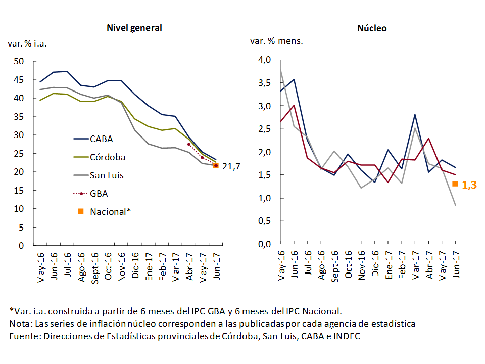
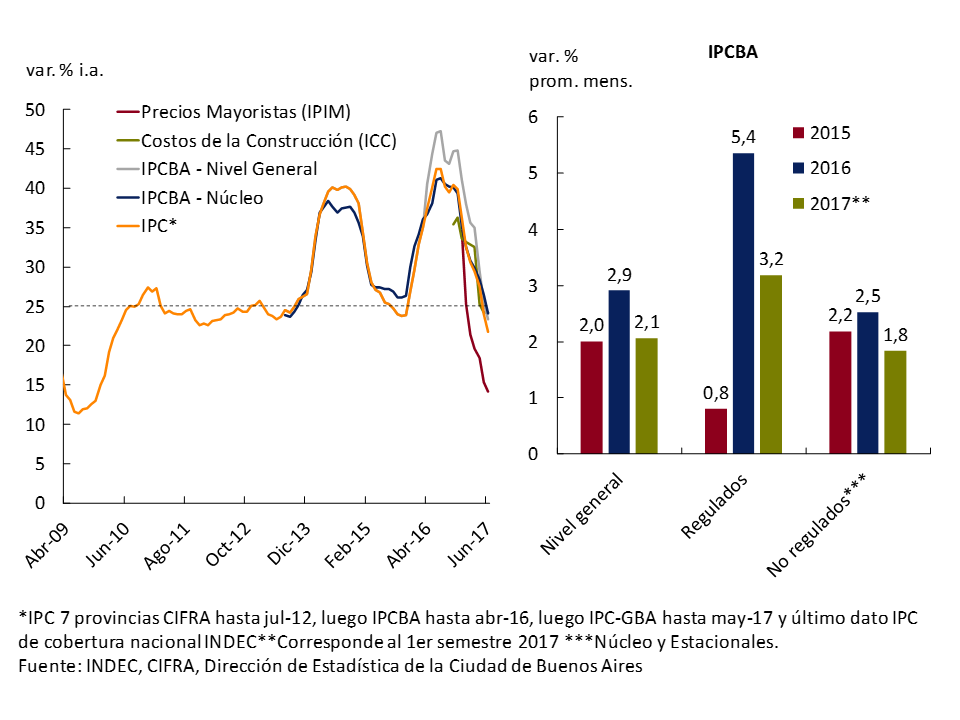
Over the last year, inflation has been systematically reduced, as can be seen in the left panel of Graph 1. So far this year, national year-on-year inflation fell from 36.6% in December 2016 to 21.7% in June 2017. This last figure arises from combining the GBA CPI until December 2016 with the CPI since January 2017. This inflation rate is the lowest since 2009. 1
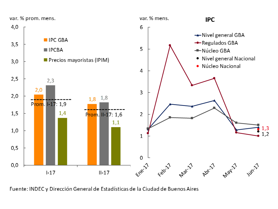
Graph 1 | Consumer Price Indices
Contemporaneous with the fall in inflation, the level of activity shows a robust recovery. July marks 11 months of growth, since the fourth quarter of 2016 GDP has grown at an annualized rate of 4%.
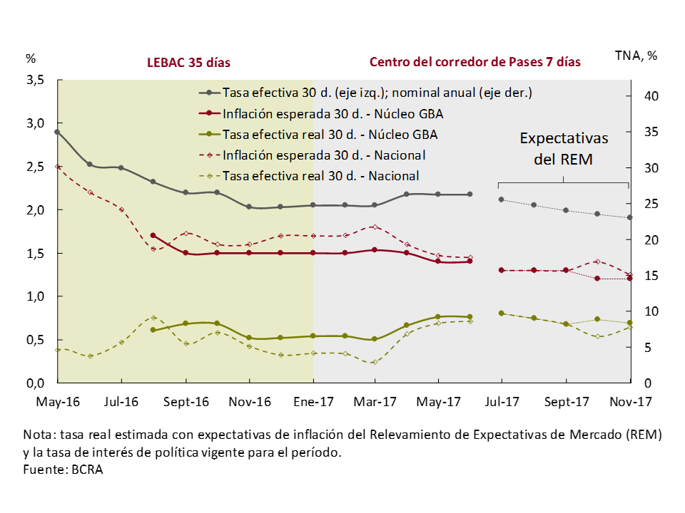
Inflation expectations, synthesized in the Market Expectations Survey (REM), show an additional slowdown to that observed in the first half of the year, with an average monthly inflation rate of 1.3% for the rest of the year. Twelve months ahead (June 2018) analysts expect a price increase of 17% and 14.9% for all of 2018. Although these are values still above the targets, it should be noted that analysts have internalized in their expectations a break with respect to the inflationary thresholds with which the Argentine economy lived for more than ten years.
The analysis of the evolution of core inflation illustrated in the right panel of Chart 1 yields three messages: a) core inflation fell sharply in the second half of 2016; b) from then on it exhibits a certain persistence; and c) in the last month, core inflation was lower than in previous months, but this evolution should be taken with caution given the aforementioned persistence.
Considering the evolution of inflation, the BCRA has kept the monetary policy rate constant since April 11 at 26.25%. However, the anti-inflationary bias of monetary policy has increased, as can be seen in Chart 2. The expected real monetary policy rate is the highest in the last 18 months (except for the atypical observation of August 2016). 2
Graph 2 | Anti-inflationary bias of monetary policy increases
The Central Bank will continue to maintain a clear anti-inflationary bias to ensure that the disinflation process continues towards its target of inflation between 12% and 17% in 2017 and that the inflation rate at the end of 2017 is compatible with the target of 10% ± 2 p.p. for 2018.
2. International context
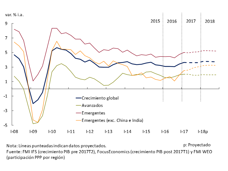
Global activity data continued to show improvement in recent months, both in advanced and emerging countries, in a context of less volatility in financial markets, although with a slight increase in the days leading up to the closing of this report. This improvement in the level of activity is partially linked to a reduction in the uncertainty factors that affected some economies. The cyclical recovery in the level of investment, manufacturing production and world trade allows us to predict that, for the remainder of the year, global economic activity will maintain the speed of growth it has shown in the first part of the year (see Figure 2.1). In the case of Brazil, Latin America’s main economy, and the first destination for Argentine exports, in the first quarter of 2017 there was a growth of 1% without seasonality (s.e.), the first after two years of recession. This occurred in the context of a disinflation of almost 8 percentage points (p.p.) in the last year and a half.
The main risks that could alter this scenario are: 1) a greater reduction in monetary stimulus than expected by the financial markets by the Federal Reserve of the United States (Fed) and other central banks of advanced economies, 2) an increase in political uncertainty in Brazil that worsens the outlook for the level of activity; 3) an escalation in geopolitical tensions, especially in the Middle East, that has an impact on global markets; and 4) the implementation of trade policies with a more protectionist tone.
Figure 2.1 | Global growth. Advanced and emerging
2.1 Recovery in global economic activity continues
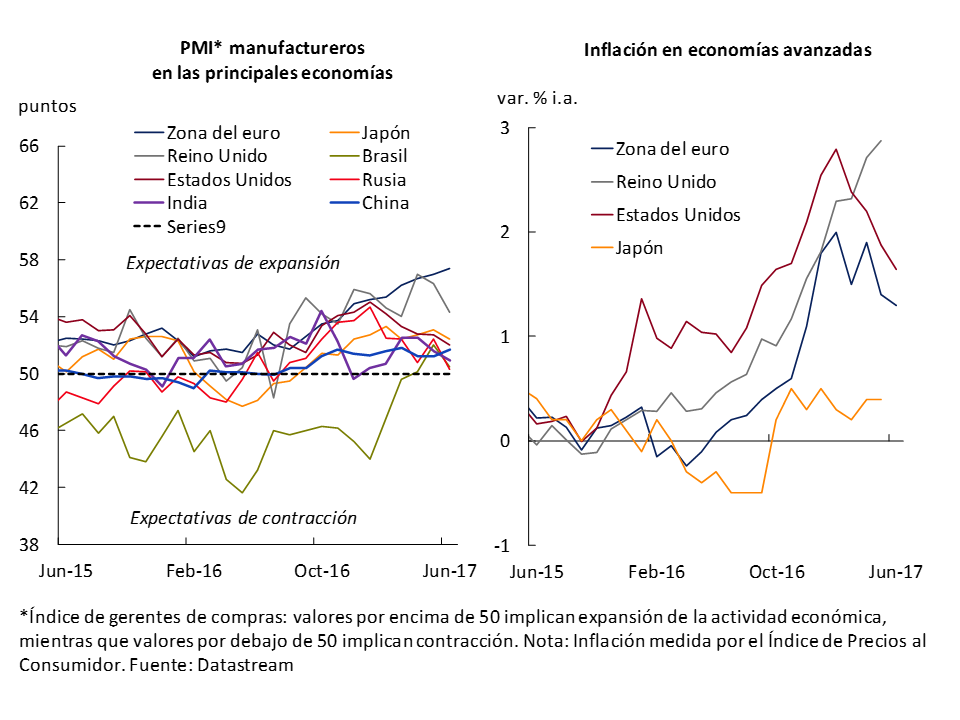
Leading indicators of activity during the first half of the year show a consolidation of the recovery that began in 2016, although with some slowdown in some countries, especially in the United States. On the other hand, throughout the second quarter, oil prices showed some downward trend, which was reflected in the inflation rate in the United States and, to a lesser extent, in the euro area, but not in the rate of change in prices in the rest of the advanced economies (see Figure 2.2).
Figure 2.2 | Leading indicators of manufacturing activity and inflation
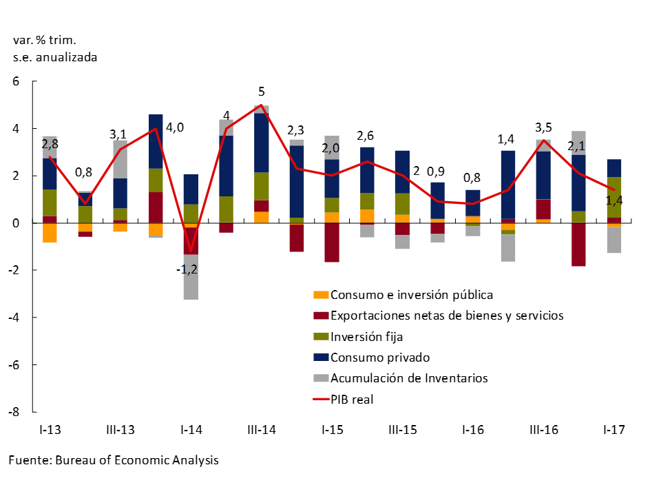
During the first three months of 2017, the U.S. economy, among the top five destinations for Argentine exports, grew by 1.4% (annualized), 0.6 p.p. below market projections. Growth was atypically driven by fixed investment with a contribution of 1.7 p.p., followed by private consumption with 0.8 p.p., while net exports contributed 0.2 p.p. (see Figure 2.3). In this context, the IMF3 reduced growth projections for 2017 and 2018 to 2.1% (a decrease of 0.2 and 0.4 p.p., respectively), mainly due to the delay in the implementation of the tax reform.
Figure 2.3 | United States. GDP growth
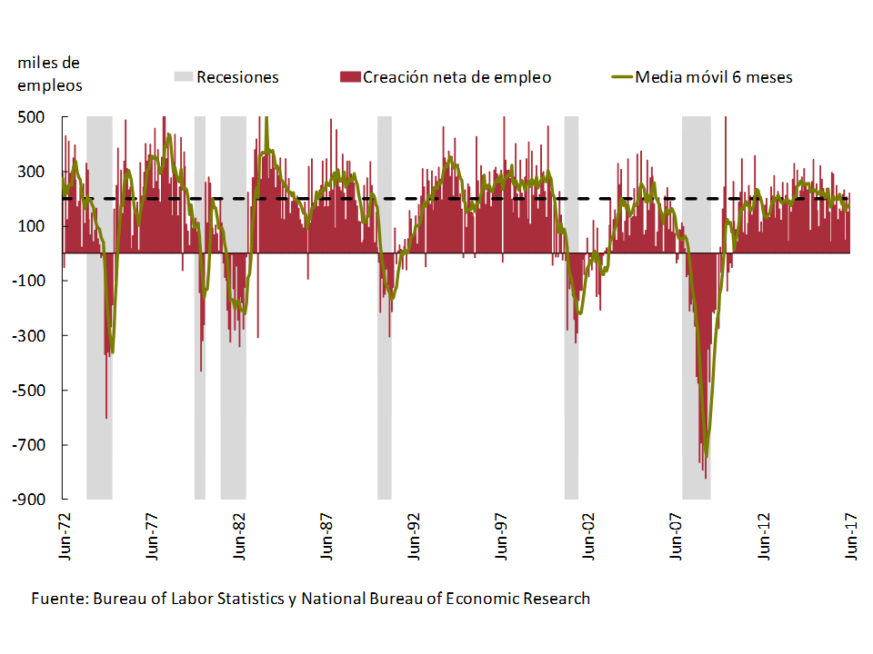
On the other hand, at its meeting in mid-June, the Fed decided to increase the target of its benchmark interest rate, the federal funds rate (TFF), by 0.25 p.p. to the range 1-1.25%. This decision was taken in a context where the U.S. economy maintained job creation close to 200,000 jobs per month (see Figure 2.4), and an inflation rate slightly below target (the rate of change of the household expenditure deflator was 1.4% year-on-year in May 2017). 4 In this context, and taking into account the statements and projections of the Fed’s Open Market Committee (FOMC)5, a further increase in the TFF target is expected for the remainder of 2017. The latter, according to market projections, would occur at the December meeting, so the U.S. benchmark rate would end the year in the range of 1.25-1.5%. Finally, in its statement from the June FOMC meeting, the Fed made it clear that it expects to start reducing its balance sheet before the end of the year. To this end, it would begin to reinvest only partially (and with a pattern of increasing cuts in reinvestment)6 the income it receives in terms of principal and interest on the maturities of Treasury securities and mortgage-backed securities.
Figure 2.4 | United States. Monthly non-farm job creation
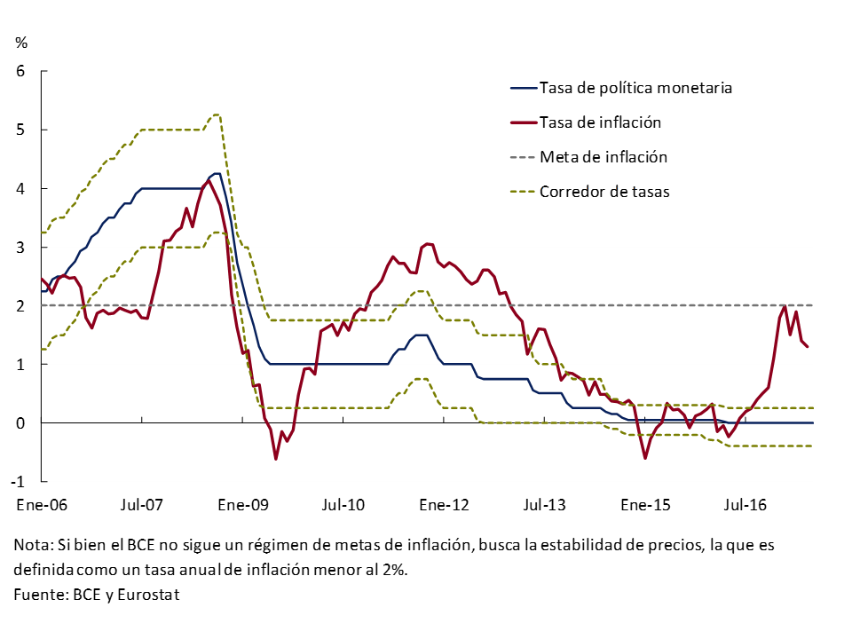
In the case of the euro area, the second destination for Argentine exports, both the growth data for the first quarter of the year and the leading indicators (see Figure 2.2) would show a consolidation of the economic recovery that began in the second quarter of 2013. In this sense, GDP grew in the first quarter of the year by 0.6% compared to the previous quarter (seasonally adjusted), which was slightly above the main forecasts. For its part, the IMF’s latest projections show that growth of 1.7% and 1.6% is expected for 2017 and 2018, respectively. In addition, the inflation rate recently increased to values closer to those desired by the European Central Bank (ECB), although with some volatility associated with movements in energy prices. In this context, at its last meeting in early June, the ECB decided to maintain its monetary policy interest rate, which it applies to Main Refinancing Operations (MRO), at an all-time low of 0% (see Figure 2.5). However, given the good outlook for the euro area, the ECB stopped including in its monetary policy statement the phrase referring to future cuts in the MRO interest rate (if economic conditions so required), thus indicating that this would no longer be a necessary measure.
Figure 2.5 | Euro area. Monetary indicators and inflation
For its part, the outlook for the Chinese economy, the third destination for Argentine exports, continued to improve, although risks associated with high levels of indebtedness and high real estate prices persist, given their potential disruptive effects on the financial system. In this regard, the Chinese authorities have accelerated the implementation of measures to deal with these risks.
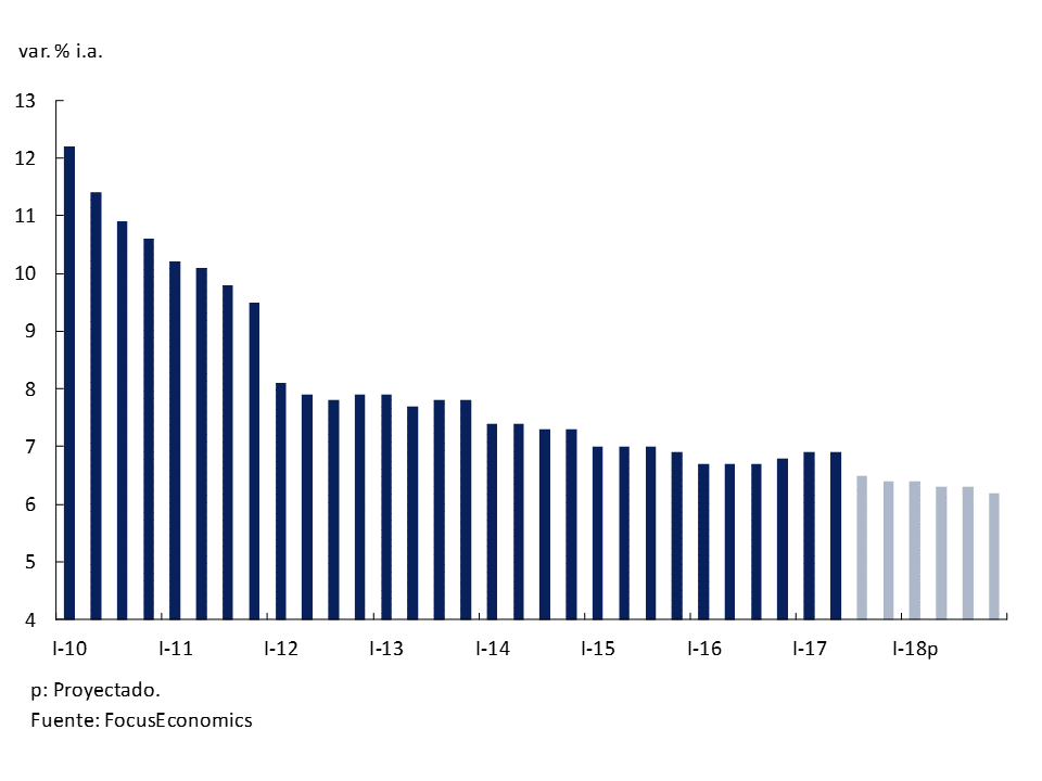
In the case of activity indicators, the Asian giant reached its growth target for 2016 (an increase in GDP of between 6.5 and 7%), and the information available to date, together with IMF estimates, suggest that these targets would also be met this year. In this regard, the activity data for the second quarter of 2017 show an expansion in economic activity, equal to that of the first quarter of the year, of 6.9% year-on-year (see Figure 2.6), while the IMF’s June projections (higher than those published in April)7 estimate GDP growth of 6.7% for this year and 6.4% for next year.
Figure 2.6 | China. GDP growth
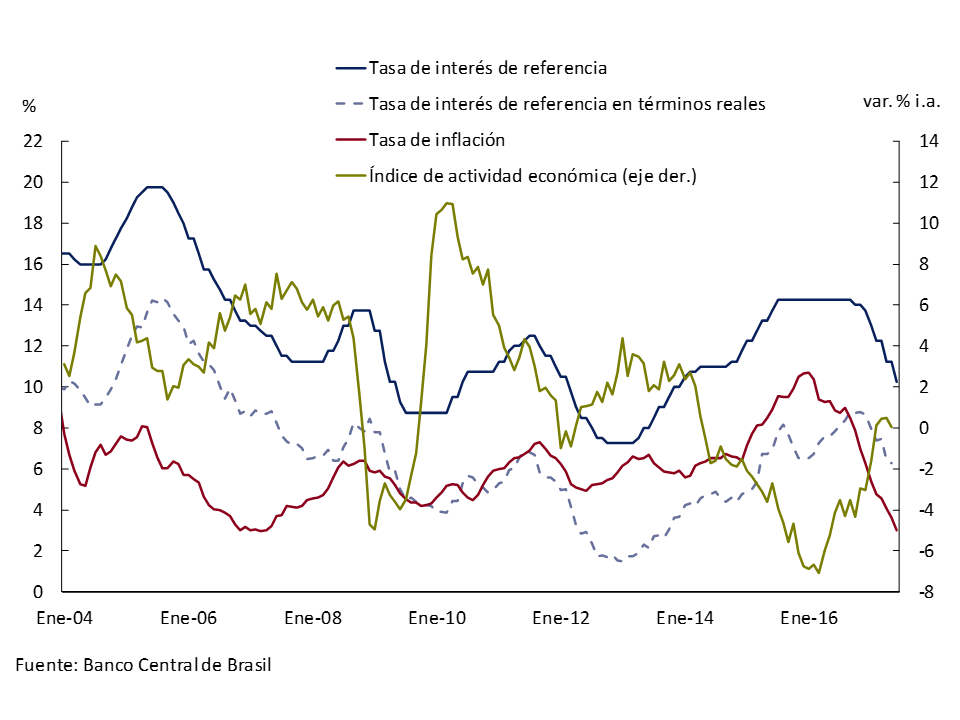
In the case of the main economy of the Latin American region, and the first destination for Argentine exports, in the first quarter of 2017, and after eight consecutive quarters of declines in the level of activity, Brazil’s GDP registered an increase of 1% compared to the previous quarter (without seasonality). Along with this, other activity indicators, such as the Economic Activity Index – carried out by the Central Bank of Brazil (BCB) – and the Industrial Production Index, began to have positive rates of change. However, unemployment levels are almost double those of 2014. In a context where a high level of political uncertainty remains, the latest projections of the Focus market expectations survey – carried out by the BCB – show that the level of activity is expected to grow in 2017 by 0.3%, and by 2.0% next year.
The inflation projections of the Focus survey indicate that a CPI rate of change of around 3.3% is expected for 2017, and 4.2% for 2018, both cases within the inflation target (4.5% ± 1.5 p.p.). 8 The latest available inflation data reflects an increase in the CPI of 3% in June, which shows a disinflation process of almost 8 p.p. in 18 months (see Figure 2.7 and box in Section 5. Monetary Policy). Therefore, the BCB is expected to continue with the process of reducing its monetary policy rate, the target on the Selic rate, which since October 2016 has maintained a downward trajectory, having been reduced by 4 p.p. to 10.25%. The specialists surveyed in the Focus survey also predict that the BCB will reduce this target by 2.25 p.p. for the remainder of 2017, so that the rate would end the year at 8%.
Figure 2.7 | Brazil. Macroeconomic indicators
2.2 Improvement and Lower Volatility in International Financial Markets
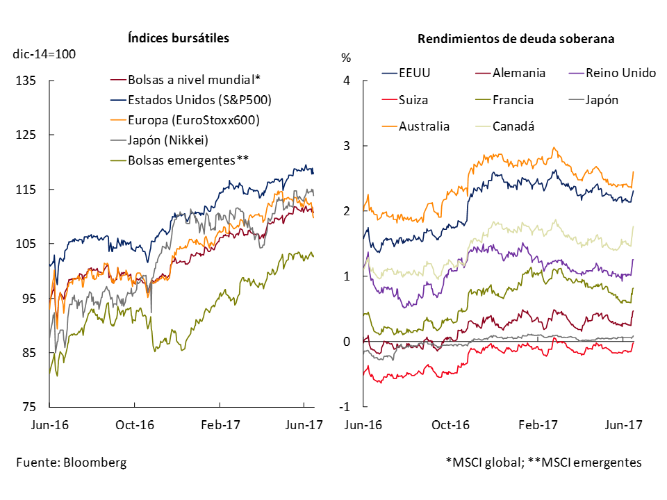
International financial markets continued a period of improvement and lower volatility following the uncertainty generated by the outcome of the U.S. elections. So much so that most stock market indicators maintained their upward path, mainly Japan’s Nikkei index and emerging market stock market indices, while yields on sovereign debt securities remained relatively constant (with a slight downward trend). However, towards the end of June, the growing possibility of a less expansionary role on the part of the major central banks (the aforementioned case of the Fed, the Bank of England, and to a lesser extent the ECB) increased the levels of uncertainty at the margin, which was reflected in the yields of sovereign debt securities (see Figure 2.8).
Figure 2.8 | Stock indices and 10-year sovereign bond yields
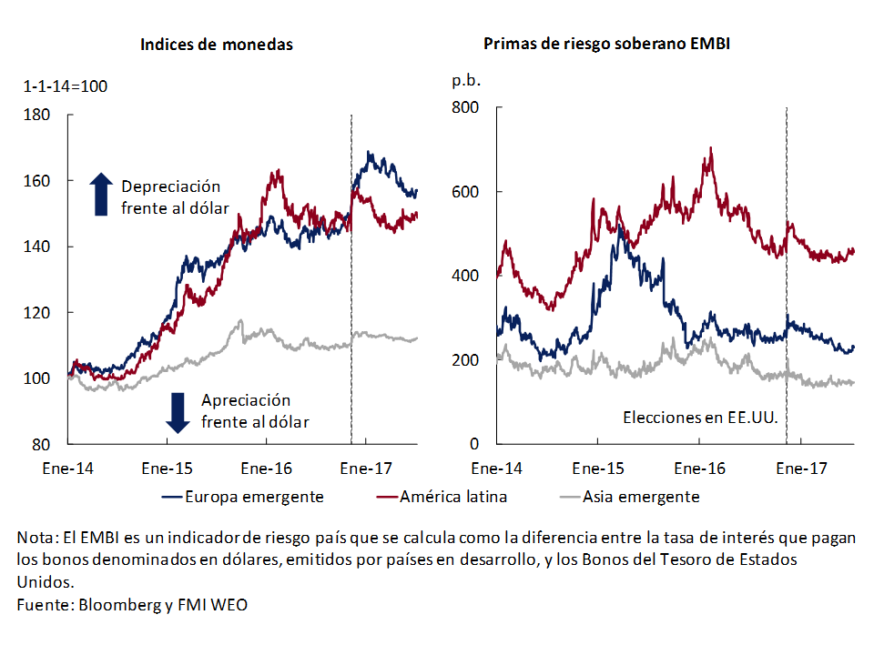
In this scenario, the evolution of the prices of the different currencies by region was uneven. On the one hand, emerging European currencies continued their revaluation process, which began once the uncertainty associated with the first post-election periods in the United States eased. On the other hand, Latin American currencies showed greater volatility in the period, partly linked to the Brazilian real and greater political uncertainty in Brazil. Sovereign risk premiums fell in almost all cases relative to pre-election values in the United States (see Figure 2.9). Like advanced economy sovereign bond yields, risk premiums in emerging Europe and Latin America increased slightly at the margin.
Figure 2.9 | Emerging. Financial indicators
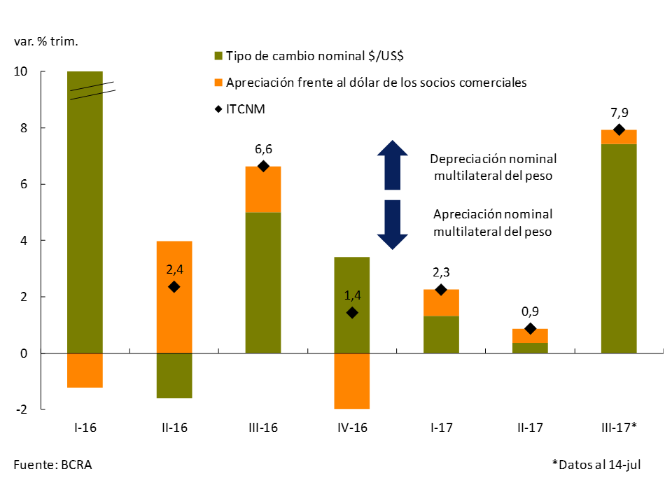
In the case of Argentina, for these indicators (exchange rate – debt securities), the Multilateral Nominal Exchange Rate Index (ITCNM) was relatively stable in the second quarter, with an increase in the first days of the third quarter (see Figure 2.10). Thus, the ITCNM increased by 0.9% (depreciation of the peso) in the first case, while so far in July it increased 7.9%. In the second quarter of the year, the depreciation of the peso is broken down into an increase in the value of the U.S. dollar against the peso of 0.35%, and an appreciation of the currencies of our trading partners against the dollar of 0.52%. While so far in the third quarter, the depreciation of the peso of 7.9% is broken down into an increase in the value of the dollar against the peso of 7.43%, and an appreciation of the currencies of our trading partners against the dollar of 0.50%.
Figure 2.10 | Change in the Multilateral Nominal Exchange Rate Index by component
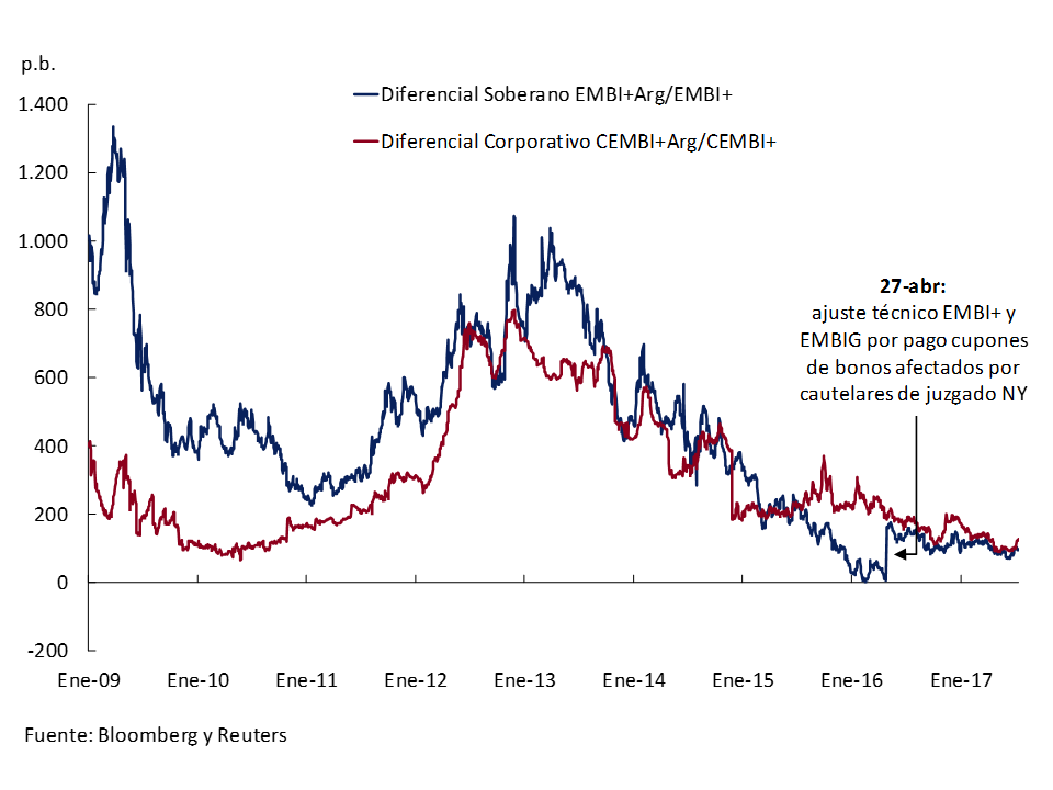
In the case of debt securities, issuance conditions in international markets for the public sector and companies improved throughout the second quarter, with a sustained reduction in the risk spreads required vis-à-vis the counterparts of the emerging countries as a whole (see Figure 2.11). In this context, there were debt placements in the voluntary markets abroad by provinces and companies, although at a slower pace than in the first quarter, while the national government managed to finance itself in June for a term of 100 years at a cost of 7.9% with an auspicious reception of offers. Three provinces obtained better financing conditions in the second quarter, to which was added a recent one, in July, by the Province of Buenos Aires, while five companies (including YPF) took advantage of these better conditions to obtain genuine financing and to improve the maturity structure of their liabilities. Thus, total financing from the public and private sectors in aggregate form in the second quarter accumulated US$5,000 million, from US$12,600 million in the first quarter. Towards the third week of June, this pattern was reversed, raising Argentina’s cost of financing, amid various factors such as the delay in the reclassification of the Argentine market within emerging markets and issues related to the political scenario in the face of the legislative elections.
Figure 2.11 | Risk premium for Argentine debt in dollars
Finally, with respect to the price of commodities, the disparate picture continued between those related to oil and the rest. In this way, the downward trend in the price of oil was maintained, which partly reflects the difficulty on the part of the Organization of Petroleum Exporting Countries (OPEC) to make effective the reduction in production announced last November. While the rest of the commodities had a more heterogeneous behavior. Thus, until June 2017, the IMF’s Commodity Price Index (where oil weighs more) fell 6.6%. For its part, the Raw Materials Price Index (CPI) BCRA – which reflects the evolution of Argentina’s main export commodities, with a marked influence on the Argentine economic cycle – fell by 2.3% (see Figure 2.10). In the case of the agricultural IPMP BCRA (where the largest amount of Argentina’s primary product exports are concentrated), a fall of 4.1% was recorded in that period.
Figure 2.12 | International commodity prices

In summary, it is expected that a sustained growth rate will be maintained at the global level in the coming months, with some stability in inflation rates, although in values slightly below the targets for advanced countries. In this context, the Fed’s monetary tightening would continue, and to a lesser extent that of the other advanced economy central banks already mentioned. In this way, monetary policy at the global level would reduce its expansionary bias, although conditions of abundant liquidity would continue to exist for emerging countries.
3. Economic activity
July marks 11 months since the recession that began in September 2015 was overcome. Since the fourth quarter of 2016, GDP has grown at an annualized rate of 4%.
The characteristics of this expansive phase shared features typically observed in the growth cycles of other countries in the region. The components of domestic expenditure (consumption and investment) accompanied GDP growth, showing higher rates of change. Net external flows were inversely correlated, with imports growing at a faster rate than exports.
The increase in GDP is consolidated, showing a more widespread growth among the productive sectors and of greater intensity.
Going forward, these trends in the economy would strengthen, processes that will allow growth of 2.7% to be achieved in the year, according to the latest estimates of the Market Expectations Survey (REM). For 2018 and 2019, the REM expects the economy to stay on track, expanding 3% and 3.2%, respectively.
3.1 Almost a year after overcoming the recession
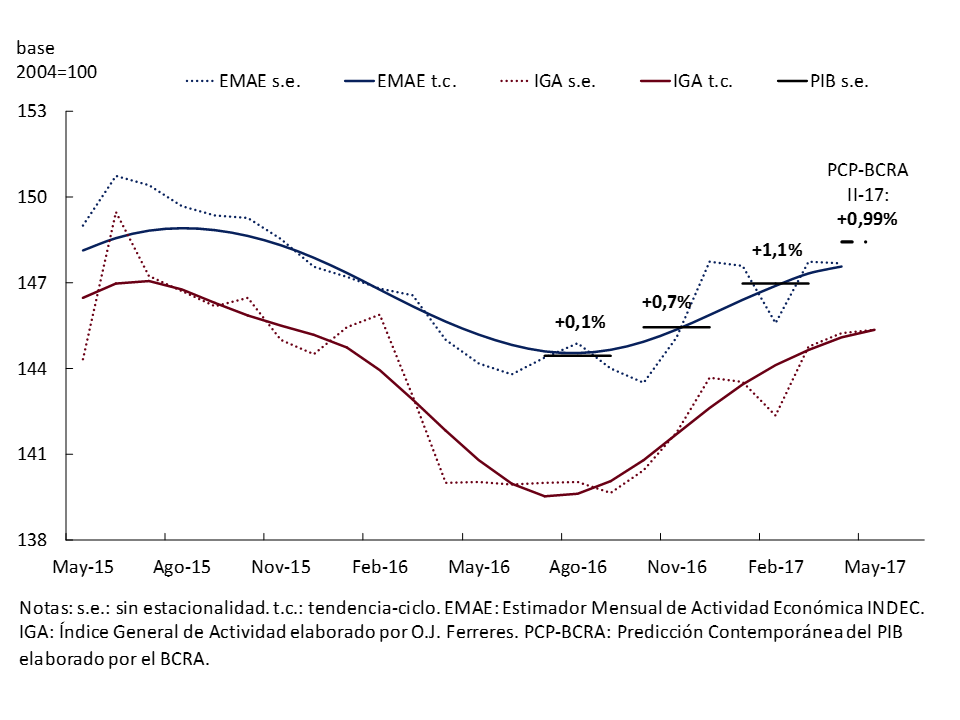
The economy continued tostrengthen9 and in June completed three quarters of growth at an annualized rate of about 4 percent (see Figure 3.1). Between January and March 2017, GDP grew 1.1% quarter-on-quarter without seasonality (s.e.), exceeding what was forecast in the previous IPOM (0.7% s.e.) and in line with REM expectations. During the second quarter, activity would have continued to expand, with the BCRA’s Contemporary GDP Forecast (PCP-BCRA; see Section 2 / Contemporary Output Prediction at the BCRA) being 1%.
Figure 3.1 | Economic activity
3.2 What is expected in the expansionary phases of an economic cycle?
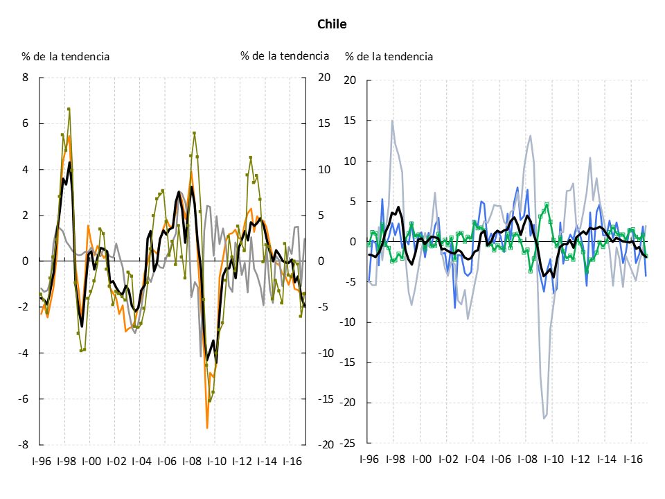
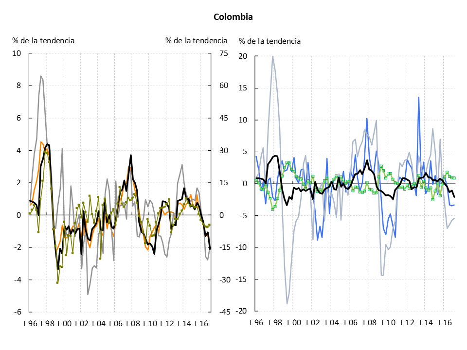
Figure 3.2 | Business Cycles in Latin America. Selected countries. Deviations from its trend
Note: The series of GDP, consumption, public consumption, investment, exports and imports of each country in the sample were calculated as the difference between the logarithm of the seasonally adjusted variable and its trend calculated using the Hodrick-Prescott filter (?: 1600). Net exports are expressed as the deviation between (a) the difference between exports and imports (divided by the GDP trend) and (b) the Hodrick-Prescott filter of (a). The series in differences of each country are composed to give rise to the joint sample composed of Brazil, Chile, Colombia, Mexico and Peru. The reference period covers from the first quarter of 1996 to the first quarter of 2017.
Source: Brazilian Institute of Geography and Statistics (IBGE) of Brazil, National Institute of Statistics of Chile, National Administrative Department of Statistics (DANE) of Colombia, National Institute of Statistics, Geography and Informatics (INEGI) of Mexico, National Institute of Statistics and Informatics (INEI) of Peru.
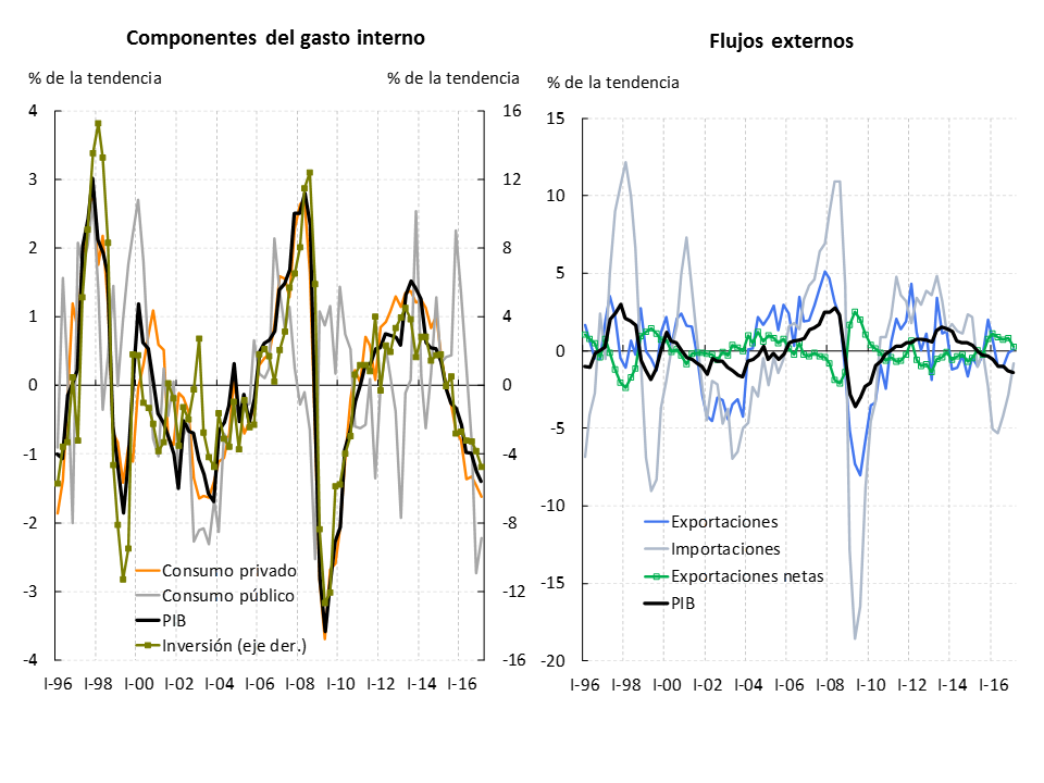
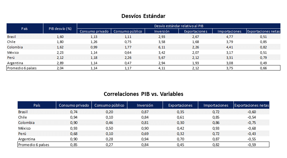
The economic cycles of the countries of the Latin American region share common features (see Table 3.1 and Figure 3.3.). From the experiences of Brazil, Chile, Colombia, Mexico and Peru between 1996 and 2017, it emerges that all the components of private domestic spending, private consumption and investment, accompany the expansive and contractionary movements of GDP and do so with greater intensity, as they are more volatile than GDP. Public consumption has a weaker correlation with the business cycle and its relative volatility differs between countries.
Looking at foreign trade, Table 3.1 and Figure 3.3 show that exports and imports are more volatile than GDP, while net external flows10 show a negative correlation with output and less variability. Typically, this occurs because as savings are more stable than investment, when investment accelerates in the expansionary phase of the cycle, net exports (which are the difference between savings and investment) are reduced.
Figure 3.3 | Business cycles. Selected countries. Deviations from its trend
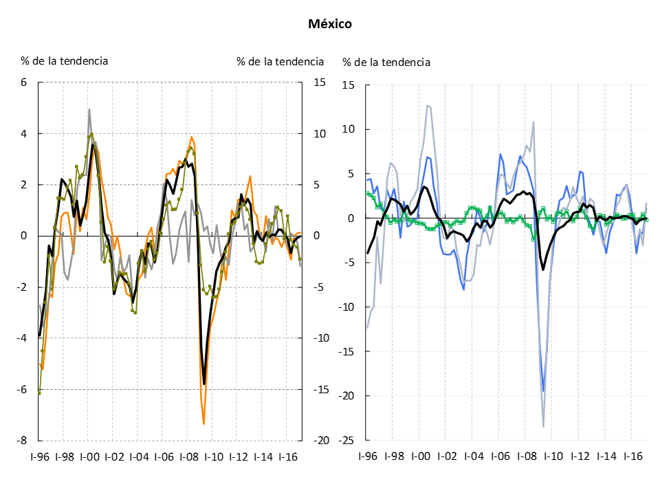
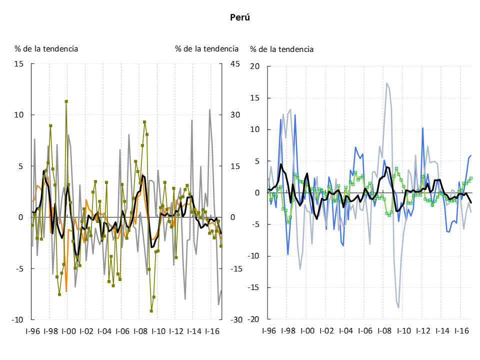
Note: The series of GDP, consumption, public consumption, investment, exports and imports of each country in the sample were calculated as the difference between the logarithm of the seasonally adjusted variable and its trend calculated using the Hodrick-Prescott filter (?: 1600). Net exports are expressed as the deviation between (a) the difference between exports and imports (divided by the GDP trend) and (b) the Hodrick-Prescott filter of (a). The series in differences of each country are composed to give rise to the joint sample composed of Brazil, Chile, Colombia, Mexico and Peru. The reference period covers from the first quarter of 1996 to the first quarter of 2017.
Source: Brazilian Institute of Geography and Statistics (IBGE) of Brazil, National Institute of Statistics of Chile, National Administrative Department of Statistics (DANE) of Colombia, National Institute of Statistics, Geography and Informatics (INEGI) of Mexico, National Institute of Statistics and Informatics (INEI) of Peru.
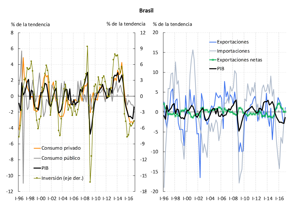
Among the components of domestic spending, private consumption and investment presented, between 1996 and 2017, a similar correlation with GDP between countries and significantly high. In Brazil and, to a lesser extent, Peru, investment showed a greater correlation with GDP than private consumption. Among external flows, imports accompanied the dynamics of the Product with greater synchrony than exports, with the correlation of the latter being the one that presented a greater dispersion among the countries under analysis.
3.3 The growth phase within the Argentina cycle
Argentina’s experience is in line with what has been observed in the countries of the region. Even both investment and exports have shown a greater correlation with GDP than their Latin American peers. Interestingly, even though exports and private consumption showed variability in line with the median of the rest of the economies and investment, public consumption and imports showed relatively low levels of volatility, Argentina’s GDP is the most volatile in the region (see Table 3.1).
Table 3.1 | Empirical regularities of cycles. Selected countries
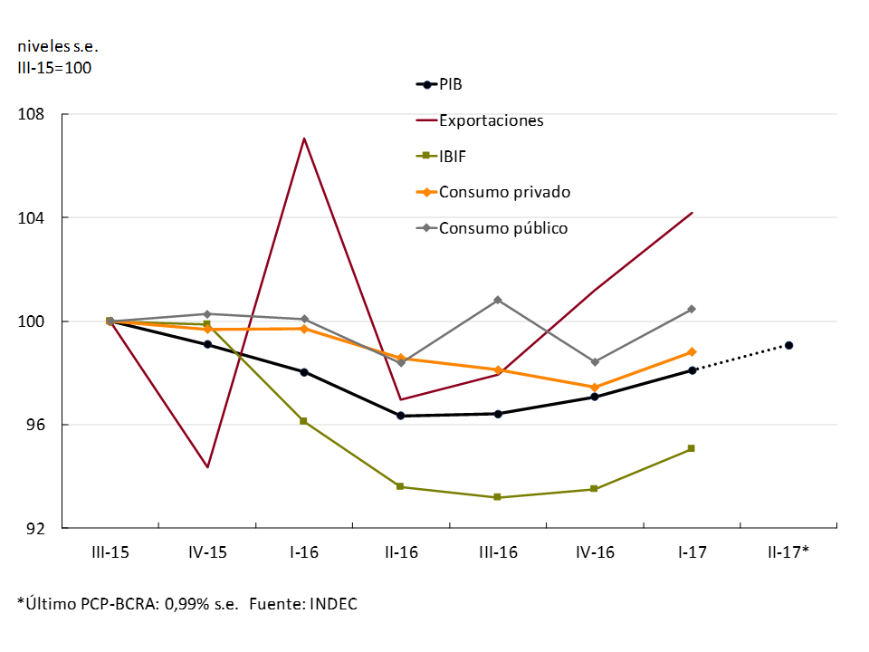
3.3.1 Unlike in other cycles, the recovery in exports preceded GDP growth
Foreign sales accumulated a growth of 7.4% in the first quarter of 2017 since the economy began to recover, outpacing the growth of the components of domestic spending. Even with the lifting of the clamps and the reduction of taxes, they had shown a recovery in the recessionary stage of the cycle, unlike the experience of the countries of the region and history itself (see Figure 3.4).
Although there are indications that exports would have temporarily stopped their growth during the second quarter of this year, they are expected to resume their growth path in the second half of the year. On the one hand, shipments of corn affected by weather conditions would resume in the first part of the year and, as sales prices in local currency improve,11 sales of the soybean complex would gain dynamism. Likewise, exports of industrial manufactures will maintain their growth trend that began in mid-2016, with a growing contribution from Brazil.
Figure 3.4 | GDP and expenditure components
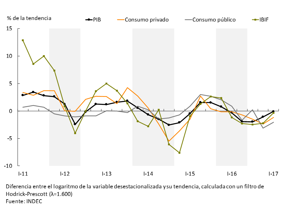
3.3.2 During the first half of 2017, higher domestic spending accompanied the growth of the economy
The growth in activity in the first half of 2017 was predictably accompanied by increases in domestic spending during this phase of the economic cycle. Strengthening consumption and investment are expected to continue for the rest of the year (see Figure 3.5).
Figure 3.5 | GDP and business cycle. Deviation from the trend
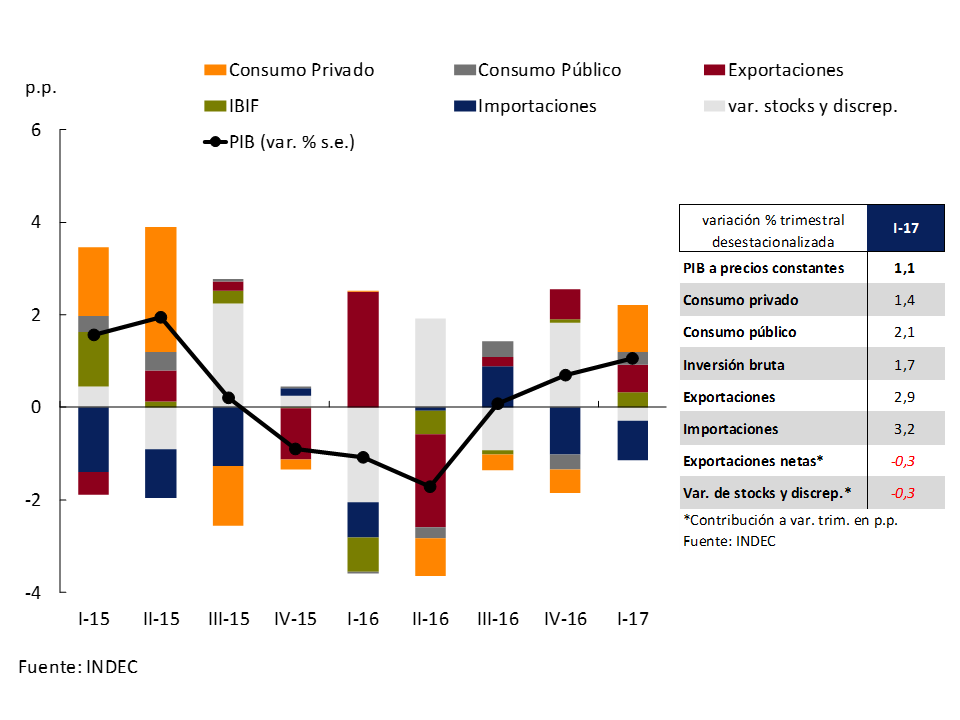
Private consumption began to reactivate as a result of the improvement in the real income of wage earners in line with the reduction in inflation observed and the rise in employment, and also the expansion of credit. In the first quarter, private consumption expanded by 1.4% s.e., contributing 1 (p.p.) to the change in GDP12 (see Figure 3.6). The improvement in the collection of gross VAT13 (3.2% between April and June), the increase in April in the quantities sold in supermarkets and shopping malls (1.3% and 1.4% monthly s.e., respectively) and the expansion of credit for families, indicate that during the second quarter private consumption would have expanded again. The Private Consumption Indicator (SSPM) prepared by the Ministry of Finance estimates a growth in private consumption of 1.2% s.e. (3.5% y.o.y.) for that period.Question 14.
Figure 3.6 | Components of aggregate expenditure. Contributions to growth
The growth of private consumption in the fourth quarter of 2016 had been anticipated by the BCRA through the Leading Indicator of Private Consumption (ILCO), a monthly index that anticipates the turning points of the private consumption series published quarterly by INDEC. The ILCO – which includes traditional indicators of the consumption of goods and services, imports, consumer expectations and indirect ways of calculating structural changes in consumption – showed a turning point in October 2016, initiating an expansionary phase since then that would continue in the second part of year15 (see Section 1 / Private consumption, a variable that is difficult to follow in real time).
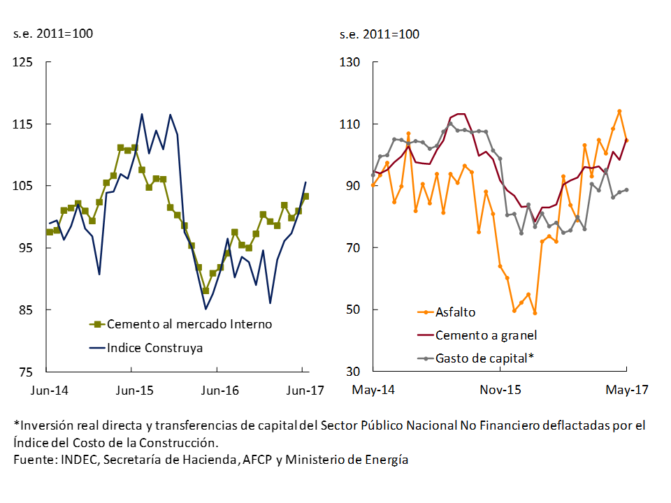
Gross domestic investment continued to recover, in line with the expansionary phase of the cycle. It grew 1.7% s.e. in the first quarter and different indicators indicate that it would have expanded again between April and June. Public works largely explained the behavior of construction in the first half of the year. Asphalt shipments for road works were among the all-time highs, with an increase of 83% y.o.y. in June 2017. In accordance with the infrastructure projects tendered in the last year, and in line with the expansion foreseen in the 2017 Budget, these works will maintain their dynamism in the coming months (see Figure 3.7).
Figure 3.7 | Investment in construction
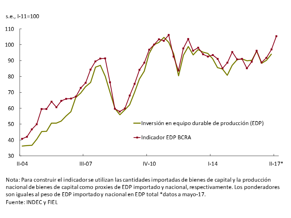
During the second quarter, private investment joined more strongly, showing signs of reactivation both in the construction segment and in durable production equipment (EDP). In relation to construction, there was a strong dynamism in cement sales in bags and a significant increase in the Construya Index, which mainly captures items associated with the completion of private works. The outlook for entrepreneurs who mainly carry out private works is mostly optimistic16 and the recovery of the sector will be favored by the BCRA’s authorization of financial institutions to accept purchase tickets and shares in construction trusts as guarantees for mortgage loans in UVA. 17 The increase in real expenditure on EDP resulted in a sharp increase in the quantities imported and a more moderate rise in the demand for equipment of national origin. Based on FIEL’s information on imports of capital goods and industrial production, investment in EDP is expected to increase during the second quarter (see Figure 3.8).
Figure 3.8 | Investment in durable production equipment
3.3.3 Imports are normalising in line with the behaviour of the cycle, after an atypical recovery in the recessionary period due to the elimination of the clamps
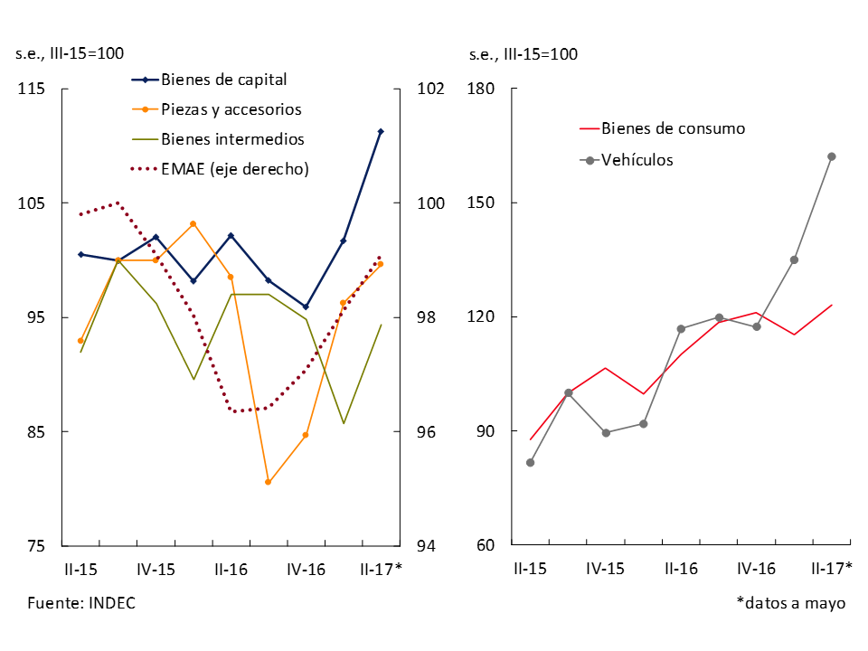
Imports increased across the board in the first half of 2017 and, unlike other experiences, have been growing since the end of 2015 since the elimination of the clamps. On this occasion, the phases of the cycle were reflected in the composition of the growth of imports. Production-related items (parts and accessories, capital goods, and intermediates) expanded during the first half of the year (see Figure 3.9).
Figure 3.9 | Imported quantities of goods
3.3.4 Growth continues to spread among the productive sectors at different speeds
During the first quarter of the year, in line with what was anticipated in the previous IPOM, the diffusion of growth among the different branches of activity increased and would have remained high during the second quarter (see Figure 3.10).
Figure 3.10 | Sectoral intensity and diffusion of growth
Box. The intensity and diffusion of growth among the productive sectors improved
Since August 2016, the economy began a recovery phase, ending the recession that began in September 2015. In order to assess the strength of the ongoing process, it is important to analyze not only its speed but also its sectoral diffusion, defined as the proportion of branches of economic activity that registered increases in their production. In a recovery phase, growth is expected to be more intense and then moderate around a long-term trend, while a greater sectoral diffusion of the expansion of activity is an indicator of sustainable growth.
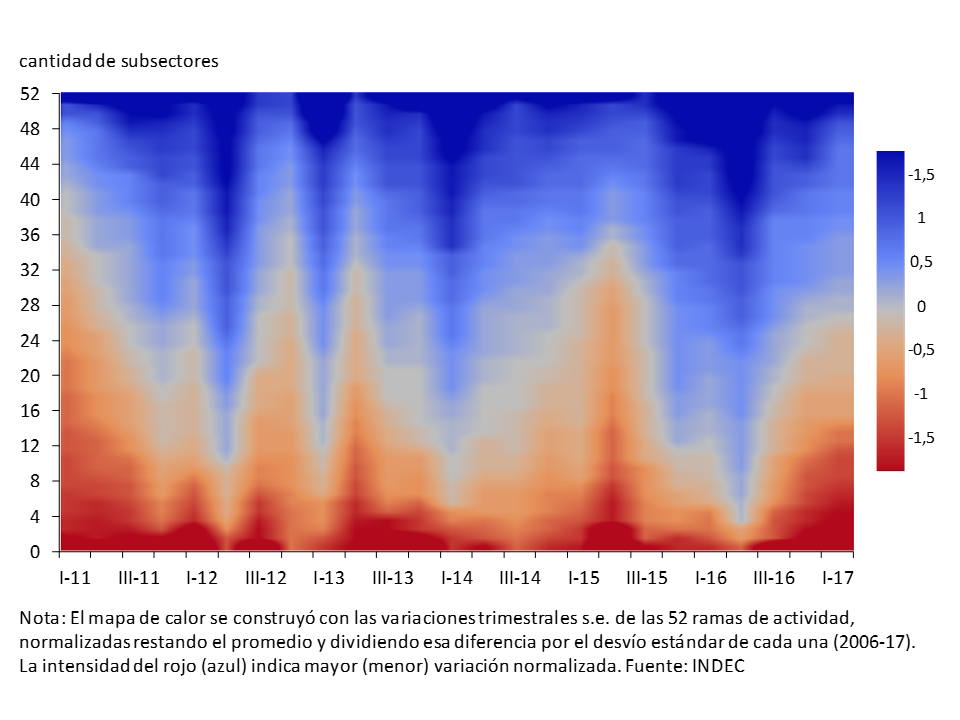
The Gross Value Added is published by INDEC in a disaggregated form into 52 branches or subsectors of economic activity. Using this information, the diffusion and intensity of quarterly growth can be calculated, although it is important to carry out some treatments prior to the series in order to make a correct analysis. To evaluate the intensity of growth, the seasonally adjusted quarterly variation of the Product of each sub-sector was compared with the average evidenced in the period 2006-2017. 18 On the other hand, the idiosyncratic characteristics make each of the series present a volatility very different from that of the rest, so it was controlled for volatility when measuring and comparing the rates of change. In summary, to analyse the intensity and diffusion, the following formula was used to normalise the seasonally adjusted quarterly variations of each sub-sector:
^g_i= frac{g_i-overset-g} {sigma}
^g_i= Normalized variation of the trim. i
g_i = variation of the trim. i
overset -g = variation trim. Average 2006-2017
sigma = standard deviation of variations
The standardized quarterly variations of the 52 subsectors of activity are presented in order of low to highest standardized growth in a ” heat map” type graph. Each subsector was graphed with red (blue) more intense the greater its quarterly increase (fall).
It can be seen that the number of branches of activity that grow around or above their average has been increasing progressively, as has the intensity of this growth (see Figure 3.10). In the first quarter of 2017, 51.9% (27) of the subsectors grew at a rate above their average, while in the second quarter of 2016 only 5.8% of them (3) did so with greater intensity.
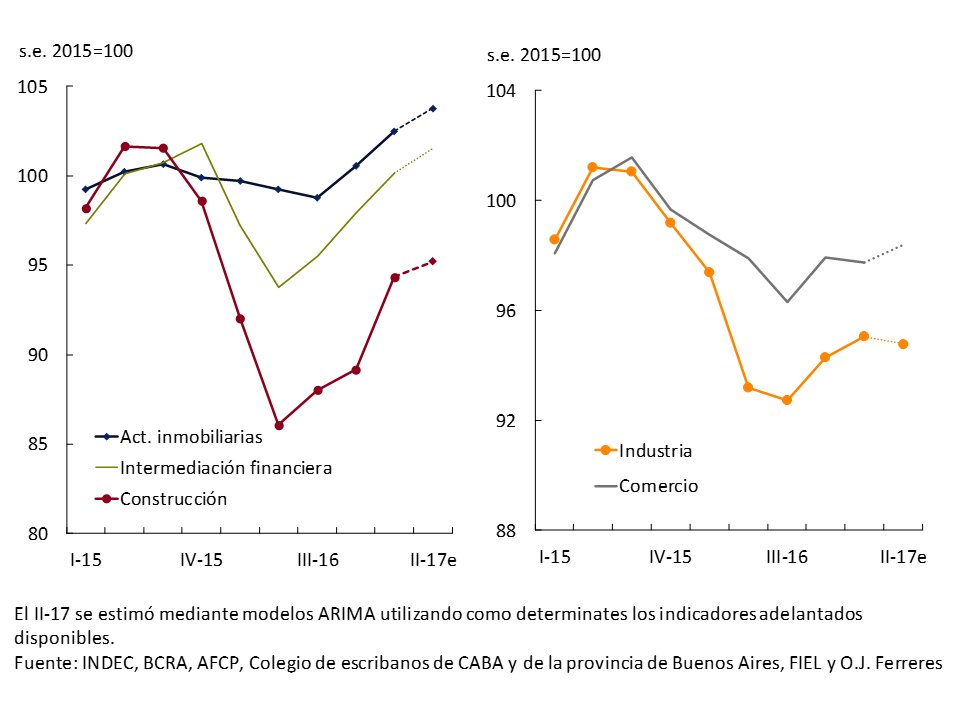
The set of policies adopted since the end of 201519 began to perform in terms of economic growth and were reflected in the sectors that led the economic recovery. Among them are agriculture, which preceded the recovery of GDP, construction, real estate, transport and communications, and financial intermediation. Another group of more moderate expansion, such as hotels and restaurants and other basic services such as education and health, accompanied the cycle. Finally, industry and commerce show a still weak recovery (see Figure 3.11).
Figure 3.11 | GDP. Main productive sectors
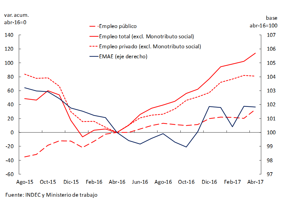
Accompanying this growth phase, in April 2017 total registered employment increased by 1% compared to the previous year. Private job creation accounted for 70% of the total increase in employment20 (73,400 workers21), in contrast to the previous employment expansion phase (Dec-14/Oct-15) in which the evolution of total employment was explained to a greater extent by the increase in public employment (54%)22 (see Figure 3.12). The number of workers in the formal private sector reversed the fall recorded during the contractionary phase, placing it slightly above the number of workers reached in November 2015.
Figure 3.12 | Employment and activity
According to INDEC, the supply of employment in the period – measured by the activity rate – was higher than the increase in demand, which is why the unemployment rate rose to 9.2%. The outlook for the next 3 months is encouraging according to the survey of job creation expectations for May by the Labor Indicators Survey (EIL) of the Ministry of Labor, Employment and Social Security.
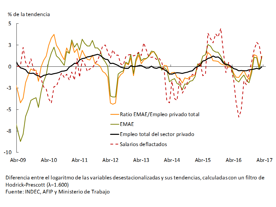
A growth rate of private employment lower than that of output is foreseeable in the initial part of an expansionary phase and denotes an increase in productivity per worker. 23 During the contractionary phase, companies usually operate by under-utilizing the labor factor through suspensions and/or cuts in hours worked. At the beginning of a recovery in economic activity, companies tend to regularize underutilization before deciding to expand their staff. Economic reforms aimed at increasing productivity will boost job creation and improve real wages (see Figure 3.13).
Figure 3.13 | Private employment, activity and real wages. Deviation from the trend
Real wages and the relative price of non-tradable goods and services improve, accompanying the economy’s upward cycle
In the second quarter, the process of recovery of real wages in the formal private sector that began in the second half of last year continued, in a context of GDP recovery and lower rates of price increases (see Figure 3.14).
Figure 3.14 | Real wages and GDP. Deviation from the trend
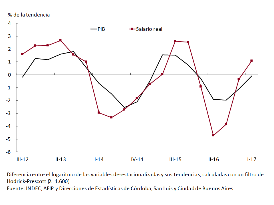
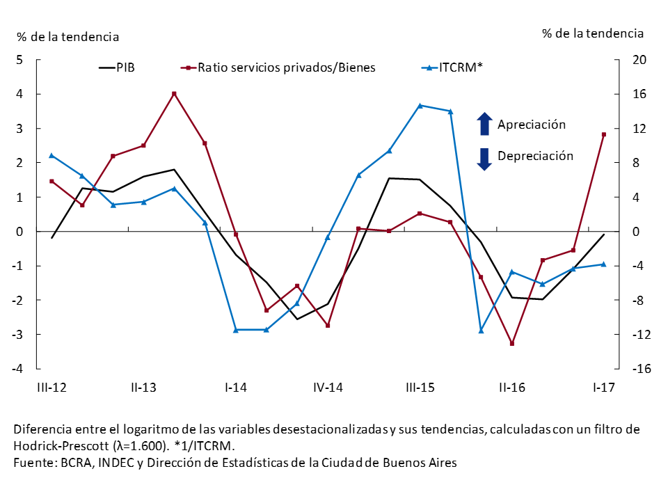
This expected behavior in an expansive phase of the cycle is correlated with the improvement in the quotient between the prices of private services and goods in the retail indices. 24 This approximation of the relative evolution of the prices of non-tradable products with respect to tradable products is in line with the appreciation of the Multilateral Real Exchange Rate Index (ITCRM) in the period (see Chart 15). The positive correlation between GDP and the real exchange rate is also corroborated in other Latin American economies (see Box).
Figure 3.15 | GDP and the quotient between the price of goods and services. Deviation from the trend
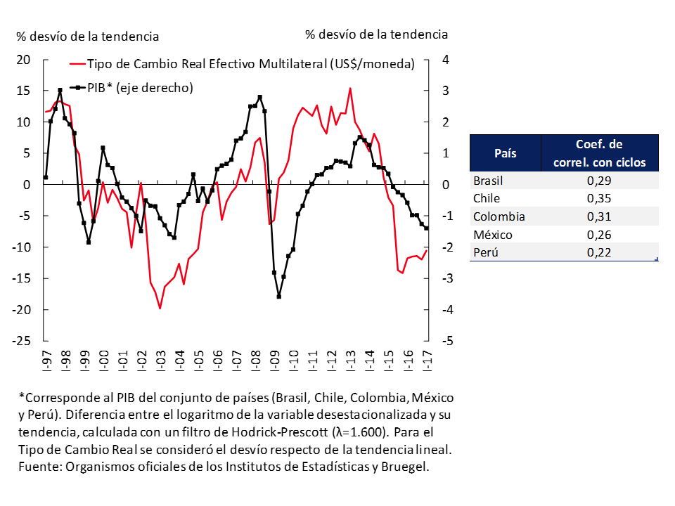
Box. GDP and Multilateral Real Exchange Rate Cycles
The economic cycles of the countries of the Latin American region share common features. For a panel of 5 countries (Brazil, Chile, Colombia, Mexico and Peru) the deviations of seasonally adjusted GDP and the Real Exchange Rate with respect to their trend were analyzed. From this information, a cycle was constructed for Latin America, which is the arithmetic average of the individual cycles. This exercise suggests that expansionary (contractionary) phases of the business cycle have a positive correlation with the appreciations (depreciations) of the multilateral real exchange rate (see Figure 3.16).
Figure 3.16 | Latin America. Selected Countries. GDP and Multilateral Real Exchange Rate (dollar/currency). Deviation from the trend
3.4 Perspectives: Well on track and with room to continue growing
The new macroeconomic configuration implemented, together with the correction of relative prices, tax reductions and the elimination of distortions that hindered the functioning of the economy, have generated widespread growth of increasing intensity.
The BCRA expects that during the coming quarters the economy will continue in the expansionary phase that began during the third quarter of 2016. This expectation is shared by the participants of the Market Expectations Survey (REM), who projected that during the third and fourth quarters of 2017 the economy will continue to expand at rates of 4% annualized (see Figure 3.17).
Figure 3.17 | REM growth forecasts
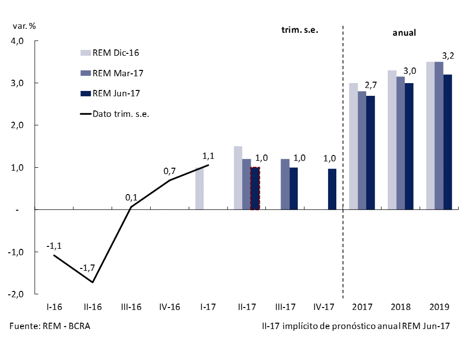
Growth would continue to spread among the different sectors of activity, boosting job creation. Exports will resume their positive trend in the second half of the year, driven by the sale of the record harvest in the agricultural sector and the recovery of demand from Brazil. The components of domestic expenditure would continue to accompany the expansion phase of GDP along with real wages.
4. Pricing
During the second quarter, the slowdown in inflation in year-on-year terms deepened, reflecting the continuity of the disinflation process that began in mid-2016. In June 2017, retail prices reached year-on-year rates of increase in the order of 22%, the lowest value since 2009.
In the second quarter of the year, average inflation was lower than that of the January-March period. However, core inflation maintained during 2017 some persistence at levels higher than those sought by the monetary authority. This behavior of core inflation is related to the dynamics of both private goods and services. The relative recovery of services, private and public, continued with respect to goods.
The expectations of analysts participating in the Market Expectations Survey (REM) remained practically unchanged from the survey available in the previous IPOM. In this framework, the Central Bank will continue to maintain a clear anti-inflationary bias to ensure that the disinflation process continues towards its objective of inflation between 12% and 17% during 2017 and that the inflation rate at the end of 2017 is compatible with the target of 10% ± 2% for 2018.
4.1 Inflation returned to the path of deceleration, after the interruption observed at the beginning of the year
During the second quarter, the slowdown in inflation in year-on-year terms deepened, reflecting the disinflation process that began in mid-2016. The different official retail indicators available expanded at a rate of around 22% YoY, the lowest value since 2009. 28 This price behavior occurred even in a process of strong readjustment of relative prices in favor of public service rates (see Figure 4.1). Wholesale prices showed a more marked slowdown with year-on-year growth rates close to 13% YoY in June 2017.
In July, INDEC began to disseminate a national CPI, which will be the reference indicator for monetary policy (see Section 3 / National Consumer Price Index). According to the new measurement, the average monthly variation in the first half of the year was 1.9%, accumulating an increase of 11.8% so far this year. These results are similar to those obtained for comparable periods in the GBA region, which has a weighting of 45% in the national total, and whose price index was the monetary policy benchmark since the implementation of the inflation targeting scheme. Within the country, the dispersion in accumulated inflation was low (1.3 p.p.29), with a very homogeneous behavior of the general level between regions.
Figure 4.1 | Inflation dynamics
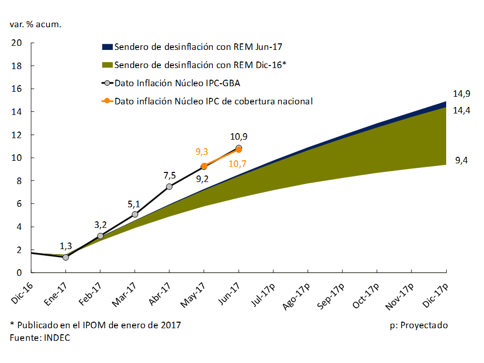
In the second quarter, prices exhibited a lower average monthly expansion rate than that recorded during the previous quarter (see Figure 4.2)30. However, the core31 measurement maintains a high persistence, although with a slight slowdown in recent months. This dynamic of core inflation is independent of the price indicator used and the methodology used to construct it. 32 Core inflation was above the disinflation path presented in the January 2017 Monetary Policy Report (MPI) (see Figure 4.3).
Figure 4.2 | Recent inflation dynamics
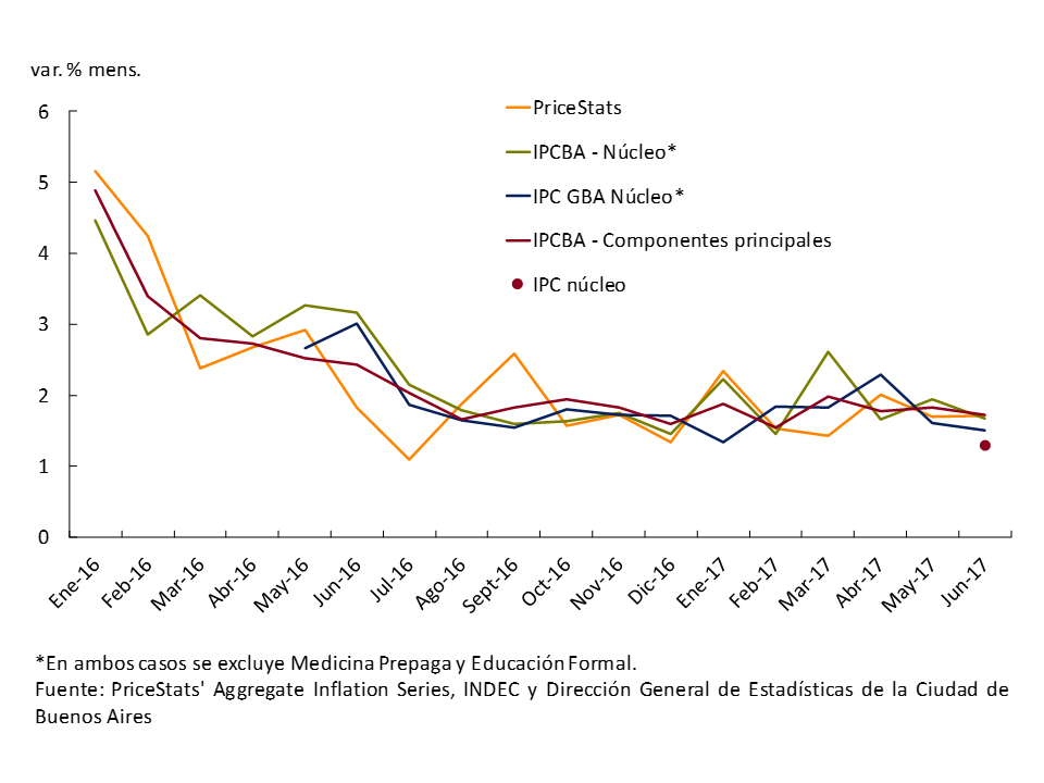
A number of available high-frequency indicators, which are more closely correlated with core inflation, also showed some persistence in their monthly growth rate (see Figure 4.4).
Figure 4.3 | Disinflation Path
Seasonal goods and services showed heterogeneous behaviors, although with a limited impact on the general price level. In the first half of the year, they accumulated a 10.1% increase in the CPI of national coverage, similar to that of core inflation.
Figure 4.4 | High-frequency and core inflation indicators
Goods registered lower rates of increase in relation to private services, in a context of greater openness of the economy. As the rate of price growth slows, those idiosyncratic movements begin to be more perceptible. The evolution of the prices of private services was consistent with the dynamics of wages in the formal private sector, given the intensity of the use of the labor factor in its production function.
Figure 4.5 | Wholesale Prices
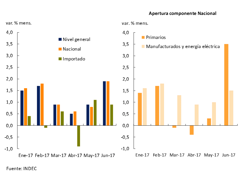
Wholesale prices33 accumulated a 7.6% increase in the first half of the year. The average growth rate in the second quarter was 1.1%, slowing down 0.3 p.p. compared to the first months of the year. The national component34 is the one that mainly explains the recent dynamics of the index. Although in May and June the nominal exchange rate depreciated at an average rate of 2.4% per month, both in the bilateral comparison with the United States and in the multilateral comparison35, the prices of imported goods increased by around 1% (see Figure 4.5). 36 The acceleration in the growth rate of wholesale prices towards the end of the quarter was linked to the behavior of primary products, mainly crude oil and gas. 37
4.2 Real wages continued to recover
In the first quarter, the process of recovery of real wages continued, accompanying the upward cycle of economic activity (see Section 3. Activity). This trend would have continued in the second quarter of the year, due to the entry of the first tranches of increase of various paritarias in a context of lower rates of price increases.
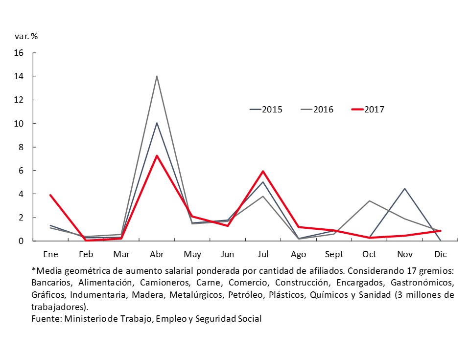
The wage negotiations closed since the publication of the previous IPOM have led to adjustments of between 20% and 24%, mostly including some type of trigger clause. This clause proved to be a useful tool to implement agreements that take into account expected inflation and not past inflation. It should be noted that, unlike in previous years, the collective bargaining agreements of the main unions38 concentrated the wage integration brackets and the largest increases in the first part of the year (see Figure 4.6).
Figure 4.6 | Salary Increase of 17 unions*
As the remaining agreements from 2016 are extinguished, new agreements that contemplate the inflation expected by economic agents for the next 12 months will come into force. In this context, it is expected to observe a progressive decline in the rate of nominal expansion of wages over the next 12 months. The continuity in the disinflation process would allow a wage recomposition to continue in real terms, associated with lower nominal increases in the general price level in the coming months.
4.3 The path of disinflation would continue in the second half of the year
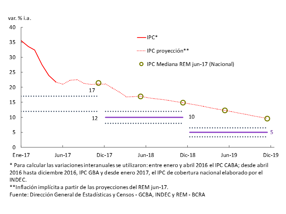
The slowdown observed in the various price indices would continue in the coming months, although in a more moderate way, as reflected in the expectations captured by the REM. For the second half of the year, market analysts forecast an average monthly inflation rate of 1.3%, lower than the first part of the year. In year-on-year terms, expectations stand at 21.6% YoY for December 2017 and 17% YoY for the next 12 months (Jun-18; see Figure 4.7). It should be noted that the deviation between the REM’s projection and the upper limit of the target remained practically unchanged from the previous IPOM (4.6 p.p.).
Figure 4.7 | Inflation Targets and Expected Inflation
In the current scenario, the main challenge will be to get core inflation back on the path of disinflation in the second half of the year. In this framework, the Central Bank will continue to maintain a clear anti-inflationary bias to ensure that the disinflation process continues towards its objective of inflation between 12% and 17% during 2017 and that the inflation rate at the end of 2017 is compatible with the target of 10% ± 2% for 2018.
5. Monetary policy
As of January 2017, the Central Bank formally adopted an inflation targeting regime, with a decreasing inflation target range over time: between 12% and 17% for 2017, between 10% ± 2% for 2018, and 5% ± 1.5% as of 2019. He also defined that to evaluate compliance with the BCRA’s annual goal, the broadest coverage index published by INDEC should be used, which is currently the National CPI that has just been released.
After nine months in which the core inflation of the GBA CPI fluctuated between 1.3% and 1.9% per month and in the face of signs that inflation in April could continue at a level higher than that compatible with the path established by the monetary authority, on April 11 the Central Bank decided to increase the monetary policy rate by 150 basis points. to 26.25%.
Although as of May the various monthly headline inflation data resumed the downward path, given that they still presented a higher trajectory than that forecast by the BCRA for this part of the year and that core inflation showed signs of persistence at values higher than those compatible with meeting the targets, the BCRA decided to keep its monetary policy rate unchanged. Having kept the nominal interest rate invariant, in a context in which inflation expectations continued to fall, the real interest rate was raised, with which the Central Bank accentuated the disinflationary nature of its monetary policy.
The Central Bank will continue to maintain a clear anti-inflationary bias to ensure that the disinflation process continues towards its objective of inflation between 12% and 17% during 2017 and that the monthly inflation rate at the end of 2017 is compatible with the target of 10% ± 2% for 2018.
5.1 Central Bank policy during the second quarter
As of January 2017, the Central Bank formally adopted an inflation targeting regime, with a decreasing inflation target range over time: between 12% and 17% for 2017, between 10% ± 2% for 2018, and 5% ± 1.5% as of 2019.
In September 2016, the BCRA had defined that the broader consumer price index published by INDEC would be used to evaluate compliance with the target, given that monetary policy aims to reduce inflation throughout the national territory, not in a particular region. At that time, the widest coverage consumer price index available was the GBA, but INDEC was making progress in the preparation of a national coverage index, which is available as of July 2017. For the first half of the year, these indices do not show significant divergences, nor are they expected to do so for the future (see Chapter 4). Therefore, in order to evaluate compliance with the BCRA’s annual target, the national CPI will be taken.
After several months in which core inflation showed no clear signs of falling (see Chapter 4. Prices) and in which headline inflation showed a higher level than that compatible with the path established by the monetary authority, on April 11 the Central Bank increased its monetary policy rate, the center of the 7-day pass corridor, by 150 basis points, to 26.25%, and has kept it unchanged since then.
Having kept the nominal policy interest rate invariant, in a context in which inflation expectations continued to show a downward trend, the Central Bank continued to accentuate the disinflationary nature of its monetary policy, raising the real policy interest rate (see Figure 5.1).
Figure 5.1 | Nominal and real policy interest rate

In order to assess the nature of monetary policy, it is useful to consider price indices that measure core inflation. These indicators are a more accurate measure of core inflation. Calculating real rates taking into account core inflation expectations reduces the fluctuations generated by changes in regulated and seasonal prices.
Inflation expectations, from the survey of expectations carried out by the BCRA with market analysts (REM), show a clear downward trajectory for the future. Analysts expect the BCRA to continue to gradually reduce its policy interest rate in the coming months, as inflation continues to decelerate, in order to maintain the disinflationary nature of its policy (see Figure 5.1).
However, expectations are not yet aligned with the central bank’s December 2017 target, but expect inflation to be at 17 percent, the upper limit of this year’s target, by mid-2018 (see Figure 5.2).
Figure 5.2 | Inflation expectations
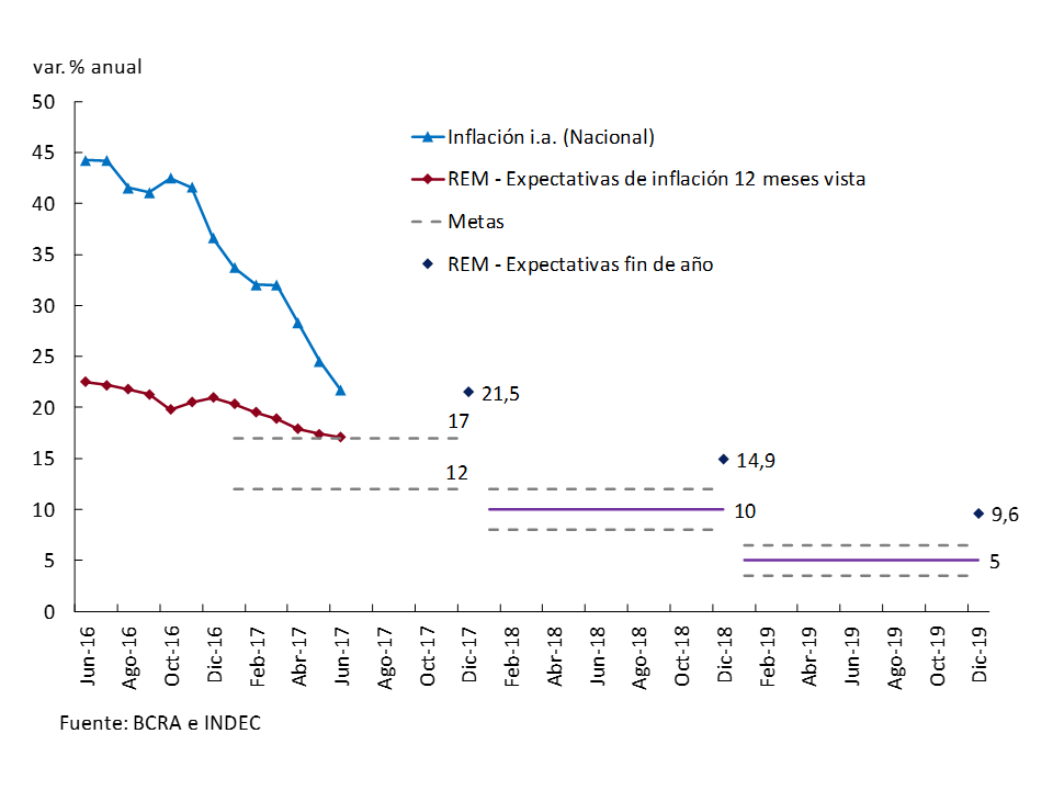
So far this year, national year-on-year inflation fell almost 15 p.p., from 36.6% in December 2016 to 21.7% in June 2017, the lowest level in the last 10 years. However, it is still 4.7 p.p. higher than the upper limit of the target range by the end of 2017.
For the coming months, the BCRA will continue to maintain a clear anti-inflationary bias to ensure that the disinflation process continues towards its objective of inflation of between 12% and 17% in 2017, and reaches during the last quarter of 2017 monthly inflation compatible with inflation of 10% ± 2% per year for 2018.
To strengthen the transmission of its policy interest rate to the rest of the market interest rates, the Central Bank returned to open market operations (OMA), through the sale of LEBAC in the secondary market. In this way, it was able to withdraw the surplus liquidity that was poured into passive passes with the BCRA, and to recover the interest rates of the LEBACs in the secondary market by 5 p.p. (see Figure 5.3), reaching values above 26% at the beginning of July.
Figure 5.3 | Interest rates on LEBACs in the secondary market
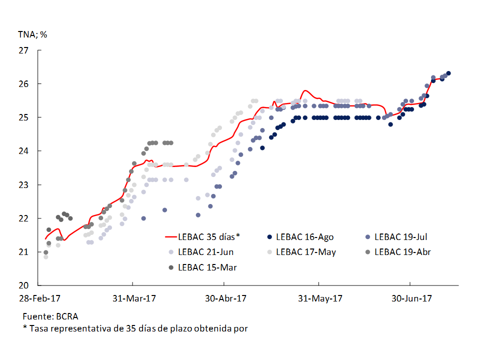
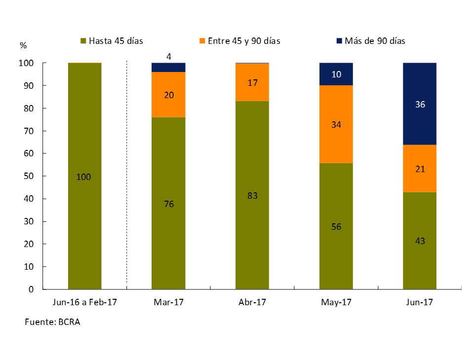
Unlike the operations carried out during 2016, when the BCRA operated in the secondary LEBAC market in the 35-day segment, to prevent interest rates from differing more than half a point from the policy interest rate (which at that time was the 35-day LEBAC auction), during 2017, its open market operations were spread across all term tranches (see Figure 5.4).
Figure 5.4 | LEBAC sales in the secondary market by term tranche
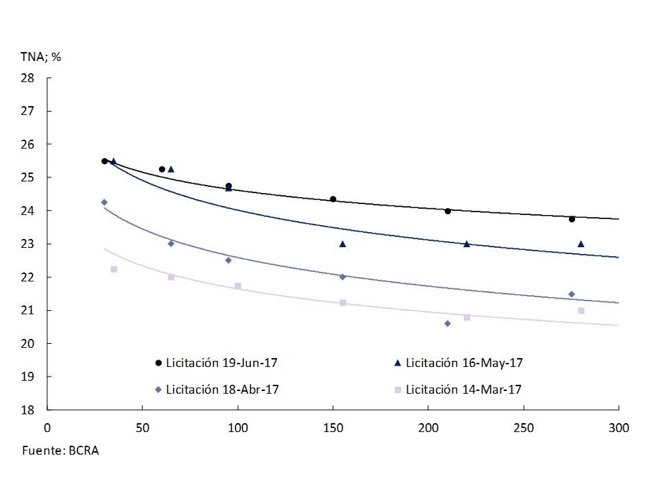
LEBAC interest rate movements were initially more pronounced in shorter-term species, so the LEBAC interest rate curve accentuated its inverted slope in April. By contrast, in May and June, interest rates on the longest species recovered the most, ending June with a more flattened slope, at levels between 3 p.p. and 3.25 p.p. above the lows recorded in March (see Figure 5.5).
Figure 5.5 | Yield curves of LEBACs in the primary market
Box: Brazil’s Recent Anti-Inflationary Experience
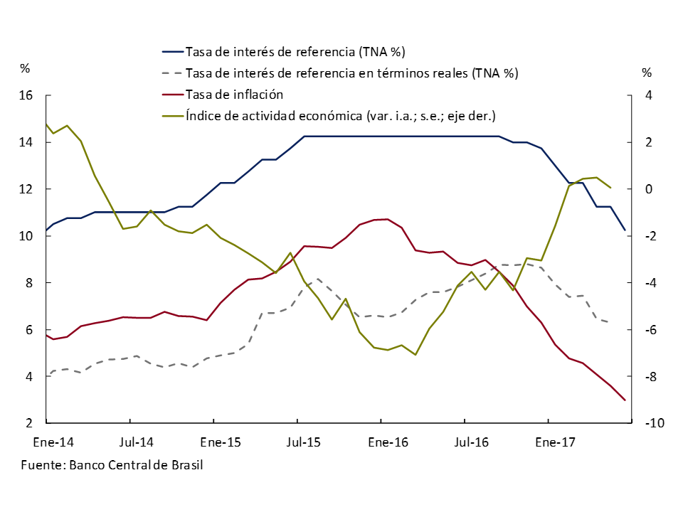
Since the end of 2014, the Central Bank of Brazil has increased its monetary policy rate, in response to the acceleration of inflation. While price growth began to show a gradual moderation in early 2016, the Central Bank of Brazil kept its interest rate invariant in order to accentuate the anti-inflationary nature of its policy.
Thus, in real terms, the policy interest rate continued to rise, reaching levels above 8%, the highest in recent years.
Thus, the process of inflationary deceleration was consolidated from year-on-year inflation of more than 10% at the end of 2015 to 3% in mid-2017, a period in which, in parallel, a recovery in economic activity began to be recorded (see Figure 5.6).
Figure 5.6 | Brazil: Policy Interest Rate, Inflation, and Economic Activity
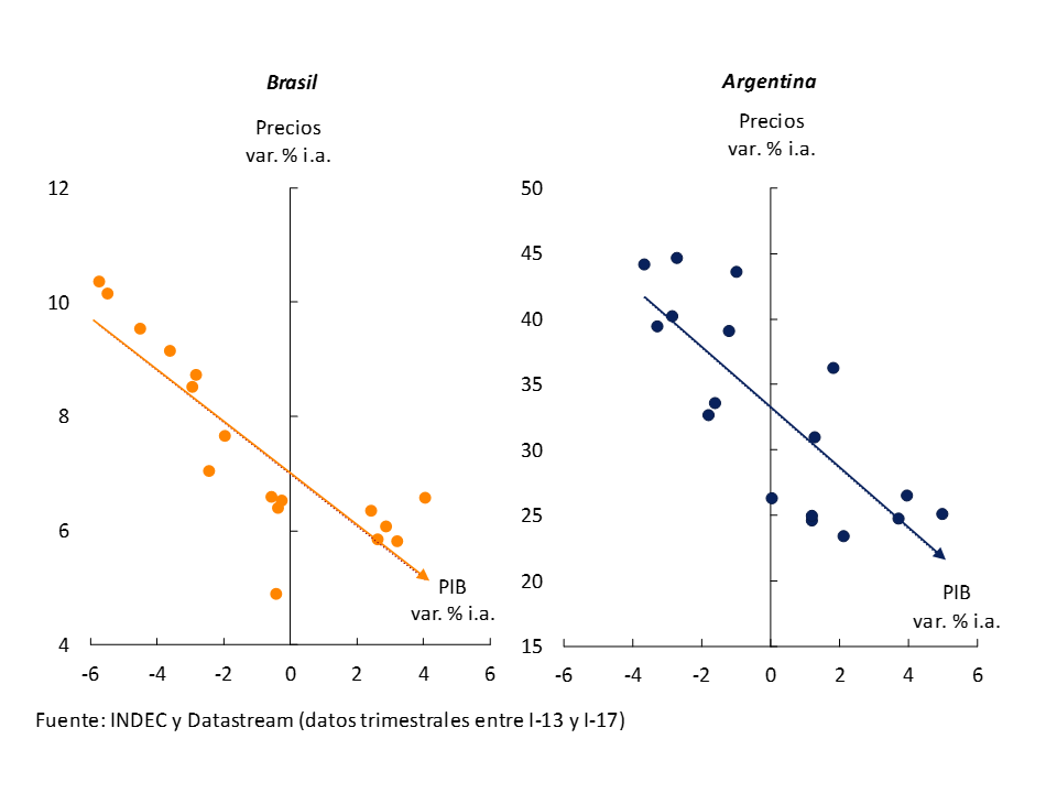
The positive effects of reducing inflation are well known. In the medium and long term, the reduction of uncertainty stands out. The disinflation process allows for a gradual extension of the time horizon on the basis of which economic agents make their savings and investment decisions. A more immediate effect is the reduction of the inflationary tax, which is highly regressive. But it is often thought that in order to reduce inflation, the growth of economic activity must be sacrificed. Recent data from Argentina and Brazil show just the opposite, that a slowdown in inflation is perfectly compatible with the growth of economic activity40 (see Figure 5.7).
Figure 5.7 | Less inflation, more growth: Argentina and Brazil (2013-2017)
5.2 The Transmission of the Policy Interest Rate to the Other Market Interest Rates
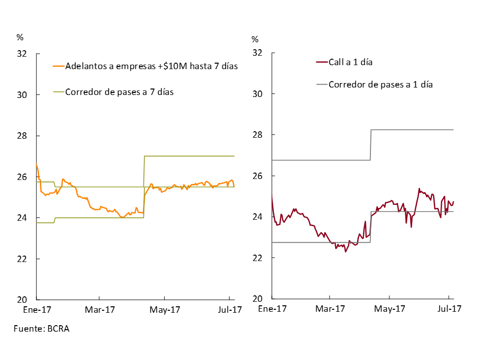
Money market interest rates registered increases, in line with the change in the policy interest rate, and were close to the new level of the pass corridor floor. In fact, the rate of advances to companies for amounts greater than $10 million and up to 7 days of term, rose around 1.5 p.p. to 25.5% in April, aligning with the interest rates of the BCRA’s passive passes with a 7-day term, while that of the interbank call with a 1-day term, it registered a similar increase to oscillate since then at around 24.5%, 0.25 p.p. above the BCRA’s 1-day pass-through rate (see Figure 5.8).
Figure 5.8 | BCRA Pass Broker and Money Market Rates
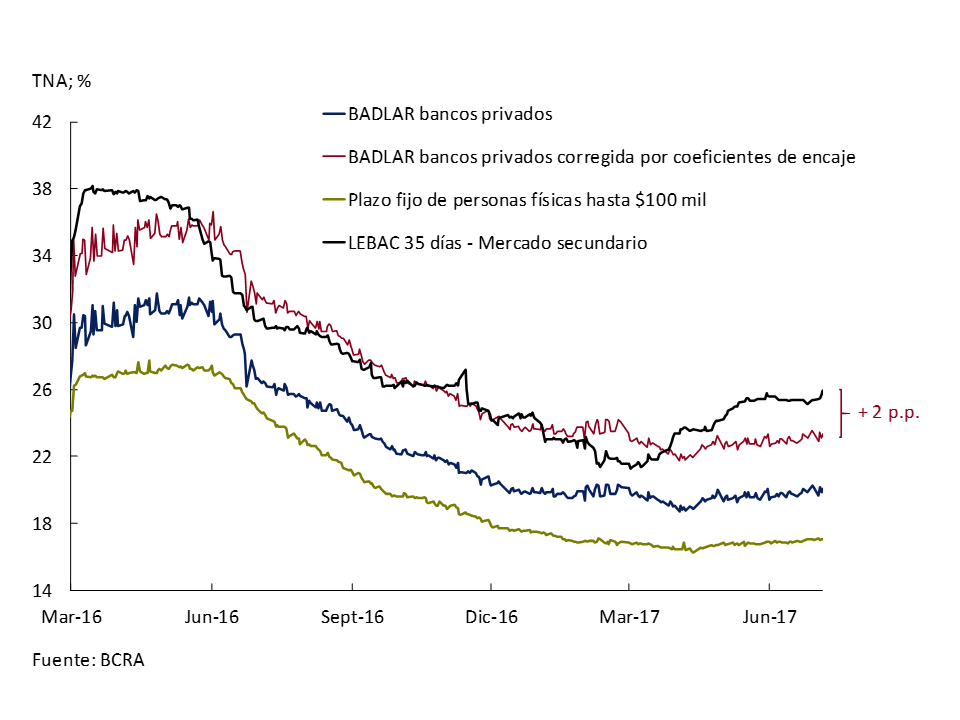
On the other hand, despite the recovery of interest rates on LEBACs, interest rates on deposits remained relatively stable. In the wholesale segment, the BADLAR remained at around 20%, registering a slight decline during March, which reversed in April, once the BCRA began to carry out open market operations with LEBAC. However, they were somewhat behind. If the funding cost of wholesale deposits adjusted by reserve requirements is compared with the 35-day LEBAC rate, it can be seen that since mid-May 2017 it has its highest spread, of around 2 p.p. In the case of interest rates on retail fixed terms, they remained around 17% (see Figure 5.9).
Figure 5.9 | LEBAC rate and bank passive rates
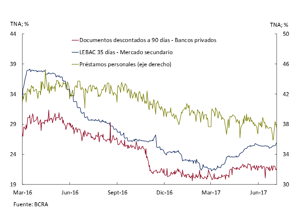
In the case of active rates, the behavior was more heterogeneous. In the case of personal loans, they continued with their slight downward trend, accumulating a decline in the second quarter of 1.3 p.p. On the other hand, interest rates on financing to short-term companies rose during the second quarter of 2017, in line with the movements in interest rates on BCRA instruments. The interest rate on discounted documents with a maturity of up to 90 days rose by 1.5 p.p. in April to stabilize at around 21.8% (see Figure 5.10).
Figure 5.10 | LEBAC rate and bank lending rates
Despite the rise in monetary policy interest rates, and some of the banks’ lending rates, credit continued to rise, as is customary in the upswing of the business cycle.
Figure 5.11 | The credit cycle and economic activity. Deviation from trend*

5.3 Accumulation of international reserves and the Central Bank’s balance sheet
Along with the decision to adopt an inflation-targeting regime, the BCRA migrated since December 2015 to a flexible exchange rate regime, which allows the economy to assimilate external shocks more naturally. However, the BCRA has been operating in the foreign exchange market occasionally, to strengthen its balance sheet, making purchases of foreign currency from both the public and private sectors, with the purpose of reaching a level of international reserves similar to that of other countries in the region that also operate under an inflation targeting scheme and a floating exchange rate regime.
The BCRA’s purchases of foreign currency from the Treasury are made when the latter must liquidate large volumes of foreign currency, and are made at the previous day’s price. On the other hand, purchases from the private sector are made by the BCRA at times when it deems it appropriate at market prices. For example, in early May, the BCRA began to make purchases in the foreign exchange market at a rate of US$100 million per day, which it interrupted when the political situation in Brazil generated greater exchange rate volatility (see Figure 5.12).
Figure 5.12 | Exchange rate and BCRA operations in the foreign exchange market
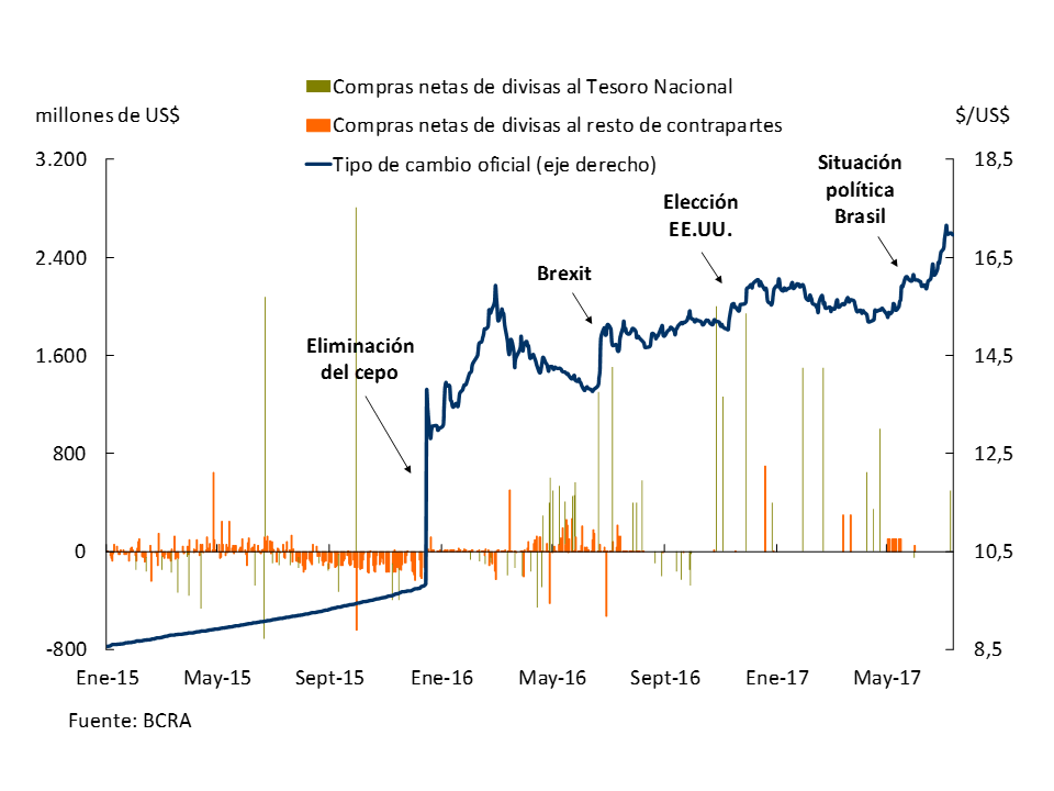
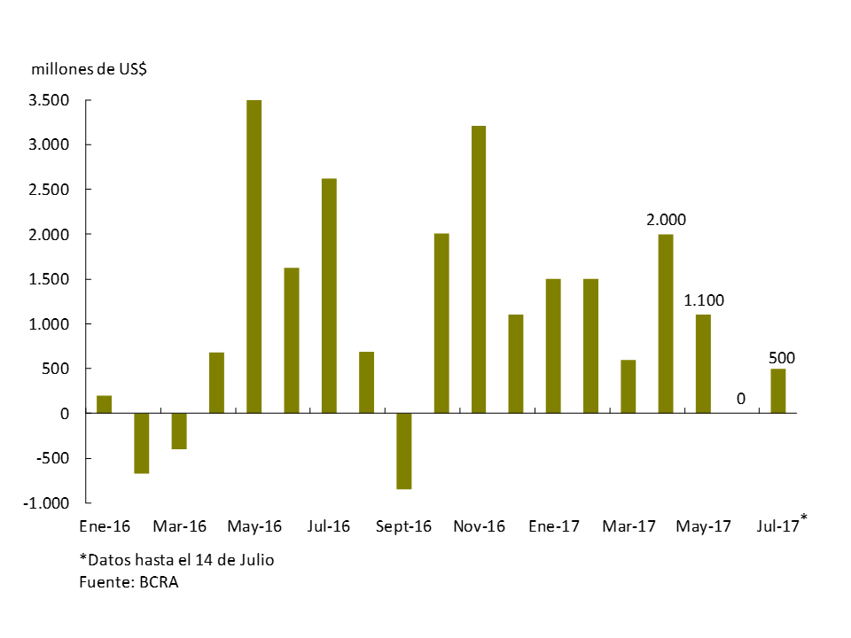
However, purchases of US$3.1 billion were made during the second quarter, and an additional US$500 million in the first half of July (see Figure 5.13).
Figure 5.13 | BCRA foreign exchange purchases in the foreign exchange market
Section 1 / Private consumption, a variable that is difficult to track in real time
In the monitoring of the situation carried out by the Central Bank, private consumption turns out to be one of the most interesting variables, although no less complex. As a result of the multiple consumption indicators that provide valuable information (even if it is partial and incomplete), it is imperative to always analyze them within a broader set of informative variables so that they acquire relevant predictive value on private consumption.
Through the use of proxy variables related to private consumption that are published prior to the quarterly National Accounts, the aim is to generate leading indicators of consumption or directly predict its behavior. Usually, market analysts link private consumption only with the demand for goods (sales in supermarkets, retail stores, shopping malls, sales of cars or appliances) without considering that services (such as transportation, housing services, health, education, leisure, etc.) have a high participation in household consumption spending. In 2016, the consumption of services represented about 60% of total private consumption while goods only 40%. 25
For these reasons, analyzing private consumption based on a single indicator, for example, sales in supermarkets, in addition to representing only a part of total consumption, can generate noisy, incomplete and partial signals that it would not be correct to generalize without taking into account a composite indicator that involves a broader spectrum of representative indicators of consumption.
On the other hand, changes in agents’ consumption habits, both cyclical and structural, pose challenges for traditional models and result in a decrease in their level of prediction. In particular, the increase in alternative or wholesale sales channels to the detriment of traditional outlets such as supermarkets; or gradual but irreversible changes in consumption patterns, such as the emergence of e-commerce26, need to be taken into account in order to model and forecast private consumption correctly.
Taking into account these considerations and discarding the seasonal, irregular effects and volatility of the original series, the methodology used in the Leading Index of Economic Activity (see IPOM January 2017) was replicated in order to detect turning points in the series and better anticipate the impact of policies and shocks on consumption.
This indicator is composed ofvariables 27 that reflect traditional measures of consumption of goods and services, imports and also indirect ways of computing structural changes in consumption. Finally, an expectations variable and another that reflects the diffusion of the growth of the whole are included. The variables that represent quantities consumed month by month were discounted for seasonal effects and receive special treatment to reduce their volatility to the minimum possible.
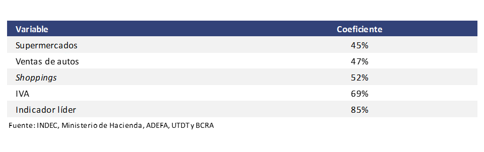
A simple comparison between the partial indicators that are usually used as anticipators of consumption and a more comprehensive one, in this case the leading indicator of consumption (ILCO), shows how the former are less accurate in keeping up with the pace of consumption. The following table shows the correlation between these indicators and private consumption in national accounts, once the series of seasonal and irregular components are filtered. As can be seen, the only one with a correlation of more than 80% is the comprehensive indicator, the ILCO.
Table 1 | Correlation with the trend-cycle of private consumption (2004-2017)
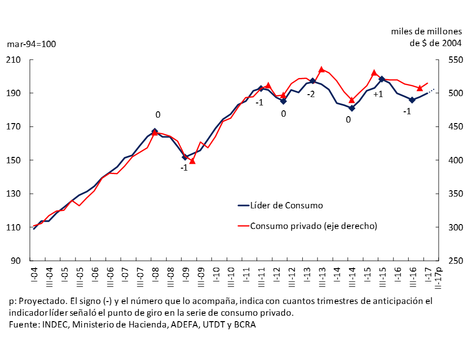
So what does the ILCO tell us about private consumption in the current situation? We know that in the 2004-2017 sample period, the leading indicator of consumption detected the turning points in the series of private consumption two quarters in advance once, with a quarter in advance on three occasions and contemporaneously twice (see Graph 1). In the third quarter of 2016, ILCO signaled a turning point that did indeed occur in the fourth quarter of 2016. Finally, for the second quarter of 2017, ILCO indicates that private consumption will continue to show positive signs.
Graph 1 | Leading Indicator of Private Consumption
Section 2 / BCRA Contemporary Output Forecasting
As of the second quarter of 2017, the BCRA Contemporary Output Prediction (PCP-BCRA) features a greater number of economic indicators with the aim of capturing the dynamics of a broader set of sectors of the economy. According to the PCP with information as of July 15, GDP registered a growth of 0.99% without seasonality in the second quarter compared to the first.
The PCP makes it possible to take advantage of the wealth of information from a large number of indicators that are published more frequently than GDP to generate output predictions within the quarter. In this way, it is possible to have advance estimates of GDP 45 days after the start of the quarter, which is published with a delay of approximately ten weeks after the end of the quarter.
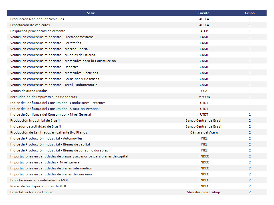
Recently, work was done on the study of new series to incorporate them into the PCP and achieve greater coverage in terms of sectors of the economy. In this process, a broad set of cycle indicators, 116 in total, were initially considered to be potentially used. These included “hard” indicators, classified as such because they convey fairly precise signals about the performance of the economy – production in industry, construction activity, trade, employment, foreign trade, monetary and financial variables, fiscal and activity in Brazil – as well as “soft” indicators, considered less accurate but with valuable information on the perceptions of different economic agents regarding the current and economic conditions. future of the economy – surveys of employment expectations, consumer confidence, among others.
To select the series to be included in the PCP, the existence of a significant contemporaneous correlation between the growth rate of each of the variables and the growth rate of activity (GDP) was used as a selection criterion. As a result, 30 series were selected from the initial potential set (see Table 1).
The methodology used to obtain the CFP, which is the same as that used in the previous estimates, is to estimate the factors common to the set of indicators of the selected cycle and to use these factors to predict GDP growth. The idea behind this methodology is that the joint dynamics of the variables of interest can be explained by a small number of unobservable factors that account for the cyclical behavior of the economy.
This set of 30 series was used to estimate the factors and, based on them, a model for the variation in GDP. It was found that the first two factors manage to explain 99% of the joint variability of the indicators considered.
Finally, the predictive capacity of the new factor model was compared in relation to the one using a smaller set of series, based on the forecast errors of both models. It was found that predictive capacity improves with the new set of information in 70% of cases – 44% in the period 2012-2015 and 92% from 2016 onwards.
Once the model is selected, the predictions are updated as new information becomes available. To do this, two groups of indicators (Group 1 and Group 2) are considered, depending on how quickly the new data is available for update (every 15 days), which allows 6 predictions of activity to be made for each quarter.
Table 1 | Series de la PCP-BCRA
According to the fifth prediction (see Graph 1), GDP exhibited in the second quarter of 2017 an increase of 0.99% without seasonality in relation to the first quarter.
Graph 1 shows the successive predictions of the PCP for the second quarter of 2017 along with information from other activity indicators available in the market, such as the O.J. Ferreres Activity Indicator (IGA) and the Monthly Estimator of Economic Activity (EMAE) of INDEC. As can be seen in the graph, 15 days after the end of the first month of the quarter, there is a first estimate of the PCP. From that moment on, the PCP provides subsequent biweekly updates of the GDP forecast for the respective quarter, which incorporate new information as it becomes available. On the other hand, the IGA provides information on a monthly basis, while the EMAE, also monthly, is published with a greater lag – at the end of the last month of the quarter (in this case June) the first activity data with information corresponding to the first month of that quarter (April) is only released.
Graph 1 | Second Quarter 2017 Forecasts
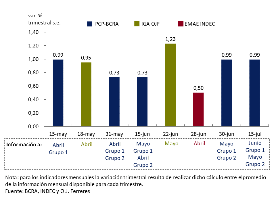
In this way, the PCP allows for a first prediction of activity in the quarter 45 days after the start of the quarter, with subsequent fortnightly updates, which implies an informative gain in terms of promptness and updating in relation to other indicators. In this sense, the CFP is a useful and valuable tool for policy decisions.
It is worth mentioning that the PCP is based on a statistical model that is automatically updated, without any intervention of expert judgment. In this sense, its results are complementary to forecasts that involve expert judgment.
Section 3 / National Consumer Price Index
In July 2017, the National Institute of Statistics and Census (INDEC) began to disseminate the Consumer Price Index (CPI) of national coverage, publishing data corresponding to the period January-June of this year. As it is the inflation indicator with the greatest coverage published by INDEC, the BCRA will use it for monetary policy decision-making, as was duly announced in September 2016 with the launch of the inflation targeting scheme.
The preparation of a CPI of national scope, following homogeneous methodological definitions for the entire territory that guarantee congruence at the regional level and its quality, allows us to have a reliable indicator of the evolution of prices representative of the entire country. The expansion of the coverage of the CPI, which until now only covered Greater Buenos Aires (CPI-GBA), is in line with international recommendations on the matter, and is therefore particularly relevant in the context of Argentina’s accession project to the Organization for Economic Cooperation and Development (OECD).
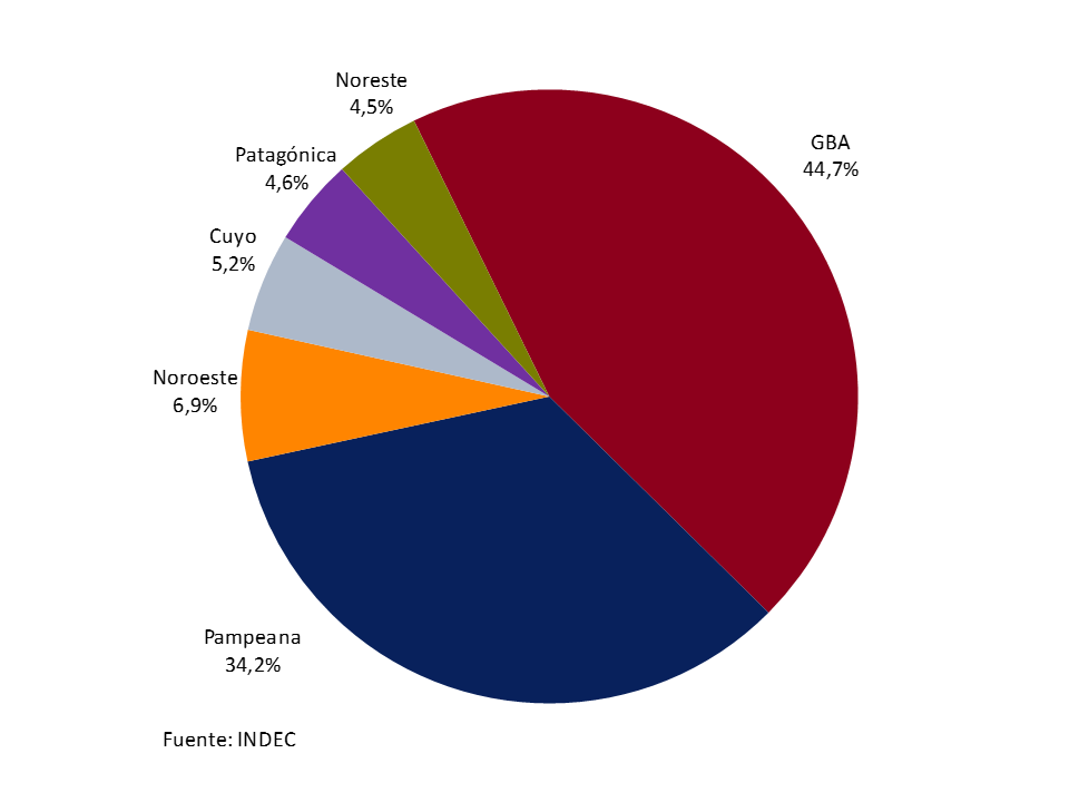
To prepare it, approximately 320,000 prices are collected per month in 40 urban agglomerations (including the City of Buenos Aires and 24 districts, which make up the GBA), covering all the provinces of the country. The price information of all the provinces, the Autonomous City of Buenos Aires (CABA) and the districts of the Buenos Aires metropolitan area is grouped into 6 geographical regions: GBA, Pampeana, Northwest Argentina (NOA), Northeast Argentina (NEA), Cuyo and Patagonica.
The CPI is constructed using a weighted average of regional indices, which are also disseminated. Each regional index participates in the CPI of national coverage according to the importance of urban expenditure in the region in total urban expenditure at the national level, according to the results of the Household Expenditure and Income Survey 2004/05 (ENGHo 2004/05). The GBA and Pampas regions have the greatest weight in the national indicator, concentrating almost 80% of the total expenditure of urban households (see Graph 1).
Graph 1 | Share of regions in urban household spending across the country
The primary information from which the goods and services that make up the basket of CPIs of each region and their weighting structure were selected was also estimated based on the information from the ENGHo 2004/05, considering the consumption expenditures of households residing in urban centers without exclusions of any kind. As in the CPI-GBA, the weighting structure of the regional baskets was updated by the evolution of prices between the reference period of said survey and the base period of the index, which is December 2015, thus reflecting the eventual changes in relative prices that occurred during that period of time.
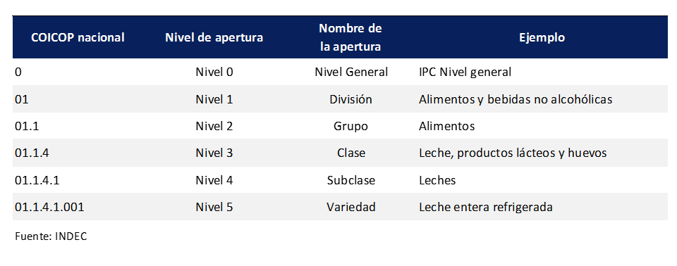
An innovation with the publication of the CPI for national coverage and the regional CPIs is the adoption of a new classifier for the basket of goods and services. INDEC began to disseminate the results of the CPIs using the United Nations Classification of Individual Consumption According to Purpose (COICOP), 1999, which constitutes an international standard.
This classifier consists of a first level of disaggregation made up of 12 divisions, which in turn are disaggregated into groups, which constitute the second level of disaggregation, and then into classes, which is the third level of openness. Up to the class level, the national classifier coincides with the international classifier, thus facilitating international comparisons, since most countries use this classifier, and also with the CPI of the City of Buenos Aires (see Table 1).
Table 1 | CPI basket disaggregation openings – COICOP Classification – Example
It is important to note that the use of different classifications to group the data does not alter the results of the general level of the index, due to the additivity property that the aggregation formula39 of the index satisfies.
The distribution of expenditure in the 12 divisions that constitute the first level of disaggregation of the new classifier makes it possible to characterize the patterns of consumer expenditure in the regions of the country. Comparing the structure of the basket at the national level with the GBA, it can be seen that expenditure in the divisions most related to services (Restaurants and hotels, Housing, Water, Electricity and other fuels, Health, Education and Transport) are of greater relative importance in the GBA than in the interior of the country. The share of Goods and Services is approximately 60% and 40% in the GBA CPI as of December 2016, respectively, while it reached 67% and 33% respectively for the CPI of national coverage (see Graph 2). In any case, the price variations shown by the CPI of national coverage in the first 6 months of 2017 are not significantly different at the aggregate level from those of the GBA CPI. While the CPI at the national level accumulated an increase of 11.8% in the first half of 2017, the GBA CPI rose 12.0% in the same period.
Graph 2 | Household consumption expenditure by purpose. Weightings as of December 2016

The structure of the consumption baskets used to prepare the CPI may not reflect current patterns. On the one hand, the weightings of the baskets are based on a survey more than 12 years ago, and the updating of the baskets by relative prices assumes that consumers did not alter their consumption patterns in the face of the changes in relative prices verified between the reference period of the ENGHo 2004/05 and the base period of the index. that is, a zero elasticity of substitution. To address this disadvantage, INDEC will carry out a new ENGHo that will provide updated information on the structure of consumption expenditures of the population throughout the country. This will make it possible to prepare a CPI that adequately reflects the current consumption patterns of the population in order to follow the evolution of inflation throughout the national territory.
Section 4 / An alternative look at the BCRA’s balance sheet
Analysing the assets of an entity is a task that can be approached according to different criteria, depending on the aspect to be evaluated. The focus may be, for example, on their level of solvency, or on the liquidity of their different assets, both in terms of their current value and in terms of what could be expected in the future, among many other variants. On this basis, this section presents a study on the BCRA’s assets from a somewhat different approach than that which would be derived from a purely accounting one.
Graph 1 shows the BCRA’s net worth expressed in41 US dollars, according to two alternative criteria. The red line reflects the institution’s net worth as it emerges from its balance sheet in each year since 2003. As you can see, it has always remained in positive values during the period in question.
Graph 1 | BCRA net worth from two different approaches (2003-2016)
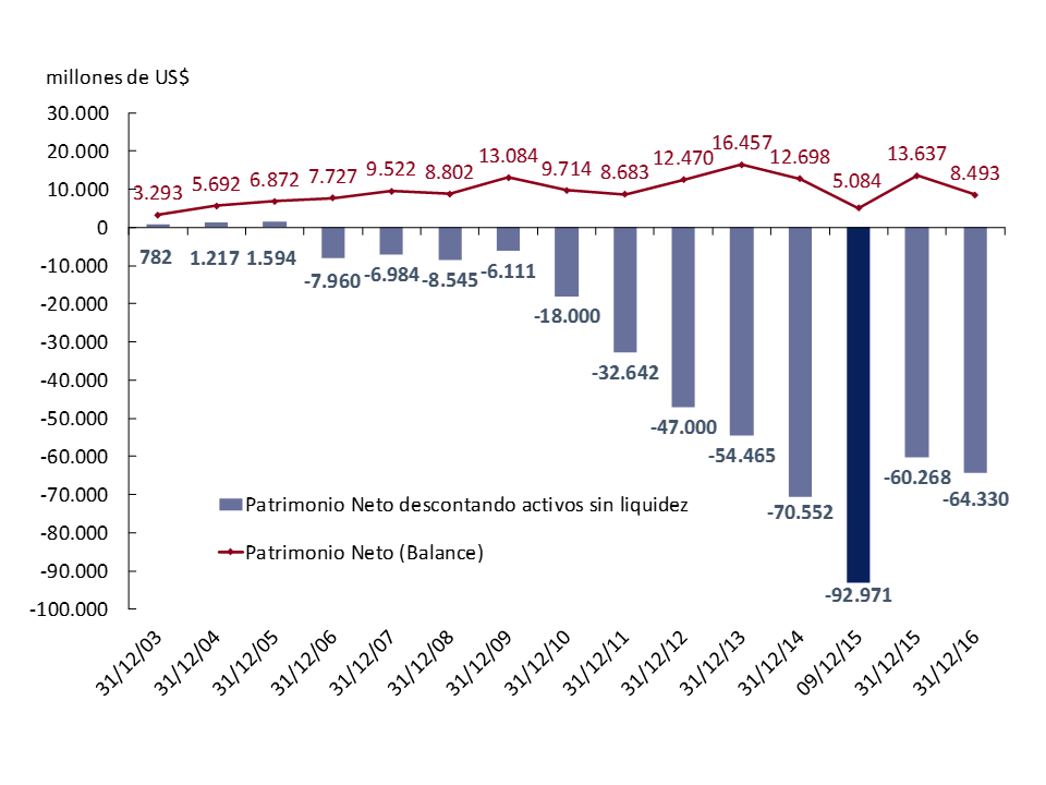
However, not all assets included in the balance sheet have the same levels of liquidity. In particular, Non-Transferable Bills (securities granted by the National Treasury in exchange for the use of international reserves) and Transitory Advances (stock of loans in pesos that the BCRA can make to the National Treasury by virtue of the provisions of Article 20 of its Organic Charter42) are computed there. A particularity that both assets share is that neither of them can be traded in the markets, so their degree of liquidity is very limited in comparative terms. It is therefore a relevant exercise to see how the entity’s net worth evolved by discounting the amount represented by these non-negotiable assets. In Figure 1, the blue bars show this alternative concept.
The graph shows that the paths over time of both measurements are radically different. According to the second approach, the entity’s net worth became negative in 2006 (due to the use of international reserves of approximately US$9,500 million to pay debts with the International Monetary Fund). Then, it maintained a certain stability until 2010, when its dynamics underwent a qualitative change and began to deteriorate rapidly. Between the end of 2009 and the time when the last change of public administration took place at the national level, it decreased by the equivalent of 86,860 million dollars. This phenomenon is mainly explained by the issuance of Non-Transferable Bills for an amount close to US$55,000 million, and an increase in the stock of Transitory Advances43 measured in dollars of 23,900 million.
In other words, the reading of the BCRA’s balance sheet varies in a non-trivial way once the public securities and loans without liquidity in the market that are accounted for as part of its assets are considered separately44. However, it should be noted that it is not technically correct to discount the entire amount represented by both securities mentioned, given that there is a probability of exchanging them for assets with greater liquidity, as was already done at the end of 2015, when the exchange of three Non-Transferable Bills of the National Treasury (the one issued in 2006 and two issued in 2010) for a value of US$ 16,000 million was carried out. in exchange for new issuances of BONAR 2022, BONAR 2025 and BONAR 2027 securities, all of which are tradable in the financial markets.
On the other hand, an additional issue that is usually ignored when analyzing the central bank’s balance sheet is the importance of seigniorage as a source of income for the monetary authority. It represents the real resources that the bank collects from the issuance of money that the public wishes to keep. It is based on the fact that the central bank issues a liability that does not pay an interest rate (and with a small marginal cost of issuance) but that is demanded by economic agents to use it as a means of payment and store of value. This income can be broken down into two factors: 1) the public’s desire to modify its demand for money (from its real balances), which depends on the interest rate and the level of economic activity; and 2) the inflationary tax, that is, the loss of purchasing power by holding money due to the effect of inflation, which represents a transfer of resources from the public to the treasury.
In this context, it is possible to propose a simple exercise of calculating the present value of seigniorage, in order to evaluate its relevance in the central bank’s accounts from a rather “economic” and not so “accounting” point of view. Considering a scenario in which the economy grows at 3% per year (which is close to the average expansion of the Argentine economy in the last hundred years), with inflation of 5% per year and with the monetary base stable at 10% of GDP (close to the current level), an annual seigniorage of 0.8% of GDP is obtained. This flow is broken down into 0.3% of GDP due to growth in the demand for money due to the expansion of the economy and 0.5% of GDP due to inflationary tax. 45 If this income is considered in perpetuity and discounted with a real interest rate of 4% per annum, the present value of seigniorage stands at 79% of GDP. 46 It can be seen, therefore, that this source of funds reaches a significant magnitude compared to the non-monetary liabilities that the central bank currently has, and shows the need to take them into account when analyzing the intertemporal sustainability of its accounts in a comprehensive way.
In conclusion, once these elements have been considered, it is possible to propose two complementary ways of approaching the study of the BCRA’s balance sheet: a purely “accounting” one (which is derived directly from the published balance sheet), and a second from a more “economic” perspective, based on what has been detailed so far. Below is the simplified result of how the BCRA’s balance sheet would look according to each approach:
Table 1 | BCRA’s balance sheet from an “accounting” and “economic” perspective (in % of GDP, as of December 31, 2016)

The table on the left is simply a summary presentation of the institution’s balance sheet, while the table on the right shows the present value of net seigniorage and the amount represented by non-negotiable assets (transitory advances and non-transferable bills) is discounted from the asset. The present value of net seigniorage is calculated from the assumptions detailed above, with a real interest rate of 4% per annum, subtracting central bank expenditures (at their current level in terms of GDP) and monetary assistance to the treasury (which converges to zero), and assuming that the discovered parity of interest rates is met at all times. As can be seen, although subtracting illiquid assets implies a marked downward correction of net worth, from the point of view of solvency the BCRA has resources that compensate (and more than compensate) for this deterioration, which is why the resulting net worth in the table on the right is notoriously higher. Even if some of the assumptions of the year are changed to generate scenarios of lower annual seigniorage, such as a reduction in the monetary base to GDP ratio to 7%, for example, due to a greater use of electronic means of payment (greater use of transactional deposits and less use of banknotes and coins), or a fall in long-term inflation to 3% per year, “economic” net worth remains at high levels (falling from 65.5% of GDP to 37.5% and 46.7% of GDP, respectively).
Paragraph 5 / Movements in the monetary base do not indicate changes in monetary policy
Since the Central Bank adopted the interest rate as an instrument of monetary policy, the quantity of money has become endogenous. Once the Central Bank determines the appropriate interest rate level to meet its inflation target, increases or decreases in the demand for money are automatically offset by movements in supply to keep the interest rate unchanged.
Although in the long term changes in the quantity of money and prices are still related, in the short term, increases in the quantity of money can respond to greater demand without this implying a risk of inflationary acceleration. This occurs, for example, in those months in which the demand for money is highly seasonal, such as that seen in June-July and December-January. In addition, during a process of inflationary slowdown, such as the one currently underway in Argentina, a strengthening of the demand for money is expected. And indeed, as of the second half of 2016, the demand for money began to strengthen (see Chart 1), which resulted in an acceleration in the year-on-year growth of monetary aggregates (see Chart 2).
Graph 1 | Balances of monetary aggregates in real and seasonally adjusted terms
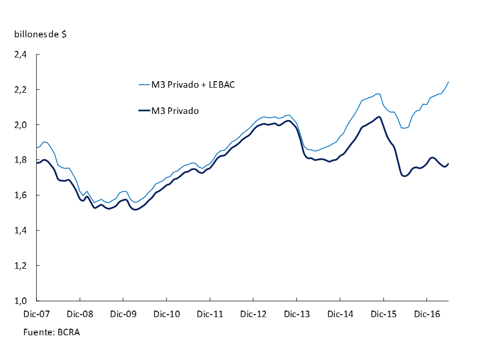
The monetary base showed a peculiar behavior, not only with a growth rate that for several months diverged from that presented by the rest of the aggregates47, but also recently presenting a more volatile trajectory within each month. To explain it, it is necessary to remember that, along with the change in the monetary policy interest rate, as of this year the frequency with which LEBACs are auctioned was reduced: the calls to subscribe these securities went from weekly to monthly.
Graph 2 | Year-on-year change in monetary aggregates

Given the flexibility provided by the reserve requirement, which must be met considering average monthly balances, the concentration of LEBAC maturities on the third Wednesday of each month and the banks’ strategy to manage their liquidity resulted in transitory expansions of the monetary base on the maturity dates of the LEBACs, which were reversed in the remaining days of each month (see Graph 3). Specifically, financial institutions partially renewed the maturities of the LEBACs, generating a surplus in their reserve position, which was offset during the rest of the month.
Additionally, in June the National Treasury placed a bond in pesos maturing in 2020, for a total of VN $75,000 million, which was settled on the third Wednesday of June, the maturity date of the LEBAC. 70% of this security was subscribed with pesos, and most of the funds for its subscription came from LEBAC. This meant that in the LEBAC auction in June, a much greater monetary expansion was observed than in previous months, accentuating the behavior described above. The result of this auction was also influenced by the seasonal increase in the demand for liquidity that occurs between the end of June and the beginning of July, associated with the collection of Christmas bonuses and winter vacations.
Graph 3 | Balance of the monetary base
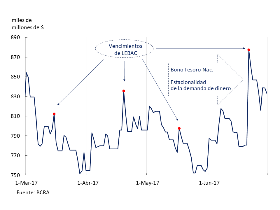
In short, all these factors give a behavior to the monetary base that should not be confused with a change in the nature of monetary policy. If the Central Bank keeps the level of its policy interest rate unchanged, increases or reductions in the monetary base do not indicate that the Central Bank has become more expansionary or contractionary.
References
1 For this calculation, the CPI 7 provinces CIFRA was considered until Jul-12, then IPCBA until Apr-16, then CPI-GBA until May-17 and the latest data of the CPI of national coverage INDEC.
2 The expected inflation in August 2016 was atypical due to the reversal of the gas tariff schedule ordered by the Supreme Court of Justice of the Argentine Nation.
3 Annual Review of the United States under Article IV.
4 The Fed does not follow a traditional inflation-targeting regime, it has a mandate to promote the objectives of “maximum” employment, moderate long-term interest rates, and stable prices. On the latter, at the meeting of the Fed’s Open Market Committee (FOMC) on January 25, 2012, a target of an annual change of 2% was set for the household spending deflator (PCE) in the long term.
5 Corresponding to the last meeting in June of this year.
6 For more details, see the corresponding Fed document published on its website.
7 April and June projections corresponding to the April 2017 World Economic Outlook and the annual review of China according to Article IV, respectively.
8 Recently, Brazil’s National Monetary Council lowered the inflation target for 2019 to 4.25% ± 1.5 p.p., and to 4% ± 1.5 p.p. for 2020.
9 The level of activity is still below potential GDP, which can be produced while maintaining a constant inflation rate.
10 Exports minus imports.
11 The external sales of the soybean complex during the second quarter were affected by the retention of soybeans by local producers in the expectation of better domestic prices. They depend on the evolution of international quotations and the exchange rate.
12 Public consumption also contributed positively (0.3 p.p.).
13 Net of refunds to grain producers and measured in real terms.
14 The Monthly Consumption Indicator of the Undersecretariat of Macroeconomic Programming of the Ministry of Finance (SSPM) is calculated from a regression model that includes the Coincident Activity Index – SSPM and the aggregation of 30 monthly frequency indicators that monitor the sales, production and/or apparent consumption of national and imported goods and services.
15 Information available as of June 2017.
16 52.6% of those surveyed believe that their activity will increase between June and August, above the percentage who expect it to remain unchanged (42.1%). INDEC, Indicators of the Situation of Construction Activity. May 2017. Vol. 1 No. 6.
17 This is in addition to the growing financing of mortgage loans in UVA. During the second quarter, financial institutions granted loans in UVA for a total of $8,667 million, of which 63.6% correspond to mortgage loans.
18 The period selected to calculate the averages and deviations of the quarterly variations in the production of the sub-sectors sought to be representative of the long-term trend growth rate of the economy. The period 2006-2017 was selected to avoid including the high growth rates 2003-2005 attributable to the post-crisis recovery of 2001-2002. Between 2006 and 2017, the economy grew at an average rate of 2.2% per year, similar to the 2.3% evidenced between 1993 and 2017.
19 Among the policies adopted are the end of exchange restrictions, the reduction and elimination of withholdings on exports, the elimination of quotas and records of export operations (ROE), the exit from default that allowed the public and private sectors access to international financial markets, the implementation of the inflation targeting scheme, the deregulation of interest rates and UVA loans.
20 The social monotax is excluded.
21 This absolute variation was 80,900 adjusting the series for seasonality.
22 In the last year (April 17/April 16), the evolution of total registered employment was explained by 69% of the creation of private employment, while public employment accounted for 31%. In contrast, in the previous expansion phase (Dec-14/Oct-15), public employment accounted for 54% of the variation in employment and the private sector for 46%.
23 At the beginning of an expansionary phase, the greater relative flexibility of hours worked in relation to jobs generates a more intense growth in output per job than in productivity per hour.
24 Estimate based on data from the CPI of the City of Buenos Aires.
25 For more details see http://www.indec.gov.ar/uploads/gacetillasdeprensa/gacetilla_consumo_privado_05_17.pdf.
26 According to data published by the Argentine Chamber of Electronic Commerce (CACE), sales through this channel represented 40 billion pesos in 2014, 68 million in 2015 and 102 million in 2016.
27 The indicator is composed of the following variables: Sales in supermarkets, sales in shopping malls, real gross VAT, sales of national cars. Credit flows with cards, imports of services, tourism, travel and tickets, flow of personal loans, ICC CABA, imports of consumer goods, commerce, hotels and restaurants.
28 For this calculation, the CPI 7 provinces CIFRA was considered until Jul-12, then IPCBA until Apr-16, then CPI-GBA until May-17 and last CPI data of national coverage INDEC. Even if we take the San Luis series, which is the only one for which historical data are available, we can see that 21.7% y.o.y. is the lowest value in the series since 2009, although this value was also reached in February and March 2011.
29 With a minimum in the Pampas region of 11.4% and a maximum of 12.7% in the Northwest.
30 There is no monthly information available on the CPI at the national level published by INDEC, the analysis of the behavior of prices throughout the semester is carried out based on data from the CPI GBA and, eventually, other official indicators.
31 It represents approximately 70% of the basket.
32 The method used by the Statistical Directorates is that of component exclusion, but other statistical measures can also be calculated by applying econometric techniques (for example: principal components and truncated means; see Section 5 of the IPOM of July 2016).
33 The basket of the wholesale price index at market prices (IPIM) is mainly composed of goods.
34 In part because of its high weighting within the index.
35 Multilateral Nominal Exchange Rate (ITCNM) with Argentina’s main trading partners prepared by the BCRA.
36 Other items such as Oil and gas that set prices in dollars also reflect the incidence of the nominal exchange rate.
37 Prices measured at the wellhead.
38 Banking, Food, Truck Drivers, Meat, Commerce, Construction, Building Managers, Gastronomy, Graphics, Clothing, Wood, Metallurgical (automotive branch), Oil, Plastics, Chemicals and Health. They make up about one-third of the workforce.
39 Laspeyres-type formula, which in the case of the CPI is P =frac{Sigma^n_{i=1} p^t_i * q^b_i} {Sigma^n_{i=1} p^0_i *q^b_i} where n are the products of the consumer basket with p_i prices and quantities q_i, 0 is the base period of prices (December 2015=100), b is the reference period for quantities arising from the ENGH (2004/05) and t is the current period.
40 See https://ideasdepeso.com/2017/04/20/desinflacion-y-crecimiento/.
41 According to the peso-US dollar reference exchange rate of each corresponding day, published by communication “A” 3500.
42 Law No. 24144 and amendments.
43 It should be recalled that the reform of the BCRA’s Charter issued in March 2012 expanded the limit for the granting of Transitory Advances to the National Treasury.
44 In line with this, it should be recalled that the BCRA will implement International Financial Reporting Standards (IFRS) for the preparation of its balance sheet as of 2018. Based on this change in methodology, its securities in the portfolio will begin to be valued at market price.
45 Although the inflationary tax is not desirable from the distributional point of view, the inflation rate for the year is at the levels shown by the economies of the region or other emerging economies, and is associated with the achievement of price stability. In addition, this level of inflation rate gives monetary policy room for manoeuvre to avoid the problem of the limit of the nominal interest rate at zero (which is not a problem for Argentina today, but could be in the future after the disinflation process).
46 The present value of seigniorage with the variables in long-run values can be expressed as follows:
VPS=frac{triangle BM}{PIB} frac{(1+g)}{(r-g)}
Where, frac{triangle BM_t}{PIB_t}= frac{(BM_t-BM_{t-1})}{PIB_t} is the annual seigniorage in terms of GDP (0.8% of GDP for all periods), r is the real interest rate (4%), and g is the growth rate of the economy (3%). The present value of seigniorage can also be expressed by considering the present value of the interest not paid for using a monetary liability minus the initial stock of the monetary base:
VPS=i frac{bm}{(1+i)}bigg(frac{1+r}{r-g}bigg) – bm
47 Several factors affected the year-on-year growth of the monetary base: changes in reserve requirements, differences in the December-February quarterly integration, and banknote logistics. For a more detailed explanation, see https://ideasdepeso.com/2017/03/22/la-tasa-de-crecimiento-de-la-base-monetaria-indica-el-sesgo-de-la-politica-monetaria/.
Glossary of abbreviations and acronyms
€: Euro
Acum.: Cumulative
AFCP: Portland Cement Manufacturers Association
AFIP: Federal Administration of Public Revenues
AUH: Universal Child Allowance for Social Protection
BADLAR: Buenos Aires Deposits of Large Amount Rate (interest rate paid for fixed-term deposits of more than one million pesos in the 30 to 35-day bracket by the average of banking entities)
BCB: Central Bank of Brazil
BCBA: Buenos Aires Stock Exchange
ECB: European Central Bank
BCRA: Central Bank of the Argentine Republic
BONAR: Argentine Nation Bond
CABA: Autonomous City of Buenos Aires
CEMBI+: Corporate Emerging Market Bond Index Plus
CEMBI+AR: Corporate Emerging Market Bond Index Plus Argentina
ECLAC: Economic Commission for Latin America and the Caribbean
CER: Reference Stabilization Coefficient
FIGURE: Research and Training Center of the Argentine Republic – Central de Trabajadores de la Argentina (CTA)
COICOP: Classification of Individual Consumption According to Purpose
CNV: National Securities Commission
Contrib.: Contribution
S Fuels Energy
DJVE: Affidavits of Foreign Sales
e: Dear
EDP: Durable Production Equipment
EIL: Survey of Labor Indicators
EMAE: Monthly Estimator of Economic Activity
EMBI+: Emerging Markets Bond Index Plus
EMBI+AR: Emerging Markets Bond Index Plus Argentina
EMBIG: Emerging Market Bond Index Global
ENGHo: National Survey of Household Expenditure and Income
EPH: Permanent Household Survey
excl.: Excluding
Fed: Federal Reserve of the United States
FIEL: Latin American Economic Research Foundation
IMF: International Monetary Fund
IMF WEO: World Economic Outlook
FOB: Free on Board (purchase and sale operations carried out by boat)
FOMC: Federal Open Market Committee
GBA: Greater Buenos Aires
A.I.: Year-on-year
IAMC: Argentine Institute of Capital Markets
IBIF: Gross Domestic Fixed Investment
ICC: Consumer Confidence Index prepared by the Torcuato Di Tella University
ICC-INDEC: Construction Cost Index
IGA-OJF: Orlando J. Ferreres General Activity Index
ILA: Leading Activity Index
ILCO: BCRA’s Leading Indicator of Private Consumption
INDEC: National Institute of Statistics and Censuses
INML: Liniers Market Steer Index
CPI: Consumer Price Index of national coverage released by INDEC
IPCBA: Consumer Price Index of the City of Buenos Aires
CPI Cordoba: Consumer Price Index for the Province of Cordoba
CPI GBA: Consumer Price Index of Greater Buenos Aires
CPI-NP: Weighted National Indicator
CPI San Luis: Consumer Price Index of the Province of San Luis
IPIB: Basic Domestic Price Index
IPIM: Internal Wholesale Price Index
MPPI: Commodity Price Index
IPOM: Monetary Policy Report
ITCNM: Multilateral Nominal Exchange Rate Index
ITCRM: Multilateral Real Exchange Rate Index
VAT: Value Added Tax
kg: Kg
LAC: Latin American Consensus Forecasts
LEBAC: Central Bank Bills (Argentina)
LFPIF: Financing Line for Production and Financial Inclusion
M2: Banknotes and coins + quasi-currencies in circulation + current accounts in $ and savings accounts in $
Mens.: monthly
MERVAL: Buenos Aires Stock Exchange
mill.: Million
Min.: Ministry
IPM: Input-output matrix
MOA: Manufactures of Agricultural Origin
MOI: Manufactures of Industrial Origin
MRO: Main refinancing operations
MSCI: Morgan Stanley Capital International Index
MULC: Single and Free Exchange Market
NEA: Northeast Argentina
NG: General level
NOA: Northwest Argentina
OECD: Organisation for Economic Co-operation and Development
OPEC: Petroleum Exporting Countries
bp: Basic points
p.p.: Percentage points
p: Projected
PAMI: Social Work for Retirees and Pensioners
PCE: Personal consumption expenditures
PCP-BCRA: Contemporary BCRA GDP Prediction
EAP: Economically Active Population
GDP: Gross Domestic Product
PMI: Purchasing Managers’ Index
PP: Primary Products
Prom. Moving Average: Moving Average
Avg.: Average
R$: Real
REM: BCRA Market Expectations Survey
REPO: Repurchase Agreement (Operación de Recompra)
ROE: Records of Export Operations
REPO Round: Average interest rate of 1-business day transactions between financial institutions in the guaranteed market
S.A: Sociedad Anónima
s.e.: Series without seasonality
SSPM: Private Consumption Indicator prepared by the Ministry of Finance
TFF: Federal Funds Rate
tonnes: tonnes
TN: National Treasury
APR: Annual Nominal Rate
Trim.: Quarterly / Quarter
ICU: Utilization of installed capacity
US$: US Dollars
UTDT: Universidad Torcuato Di Tella
UVA: Unit of Purchasing Value
Var.: Variation
Vol.: Volume
YPF SA: Yacimientos Petrolíferos Fiscales Sociedad Anónima
Share on


