Summary
As indicated in its Organic Charter, the Central Bank of the Argentine Republic “aims to promote, to the extent of its powers and within the framework of the policies established by the National Government, monetary stability, financial stability, employment and economic development with social equity”.
Without prejudice to the use of other more specific instruments for the fulfillment of the other mandates – such as financial regulation and supervision, exchange rate regulation, and innovation in savings, credit and means of payment instruments – the main contribution that monetary policy can make for the monetary authority to fulfill all its mandates is to focus on price stability.
With low and stable inflation, financial institutions can better estimate their risks, which ensures greater financial stability. With low and stable inflation, producers and employers have more predictability to invent, undertake, produce and hire, which promotes investment and employment. With low and stable inflation, families with lower purchasing power can preserve the value of their income and savings, which makes economic development with social equity possible.
The contribution of low and stable inflation to these objectives is never more evident than when it does not exist: the flight of the local currency can destabilize the financial system and lead to crises, the destruction of the price system complicates productivity and the generation of genuine employment, the inflationary tax hits the most vulnerable families and leads to redistributions of wealth in favor of the wealthiest. Low and stable inflation prevents all this.
In line with this vision, the BCRA formally adopted an Inflation Targeting regime that came into effect as of January 2017. As part of this new regime, the institution publishes its Monetary Policy Report on a quarterly basis. Its main objectives are to communicate to society how the Central Bank perceives recent inflationary dynamics and how it anticipates the evolution of prices, and to explain in a transparent manner the reasons for its monetary policy decisions.
1. Monetary policy: assessment and outlook
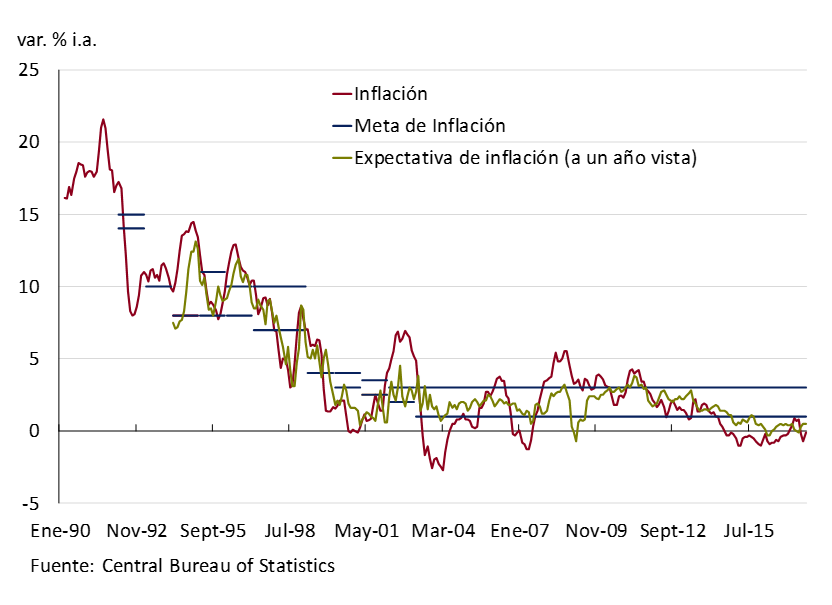
The inflation targeting regime launched in September 2016 has made it possible to consolidate for the first time in a long time an expectation of declining inflation for the next two years. The targets are 10% ± 2% in 2018 and 5% ± 1.5% in 2019. Despite this substantive achievement, challenges remain regarding the pace of the disinflation process, which continues to be above that sought by the monetary authority.
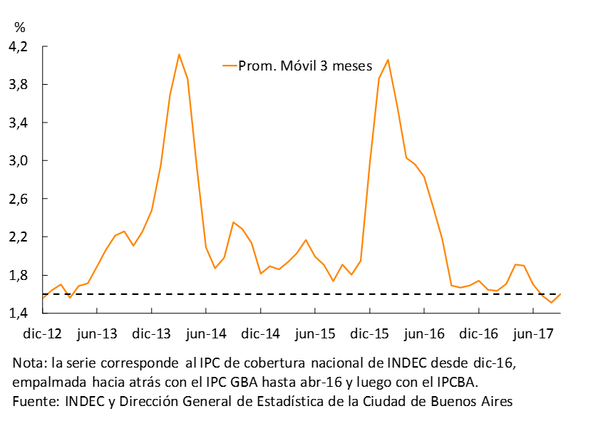
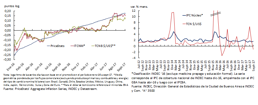
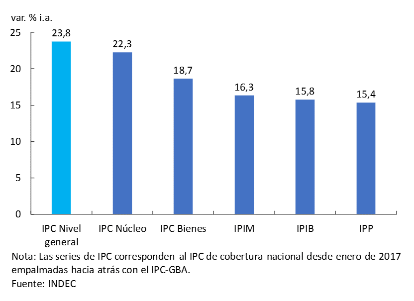
During the third quarter, inflation stood at 1.7% monthly average, falling marginally compared to the 1.8% of the second quarter. This is the lowest quarterly inflation rate, at the three-month moving average, since May 2011. There was also a greater regional dispersion in the comparison against the first two quarters of the year. Year-on-year inflation, meanwhile, fell to 22.7% (III-17) and is practically half of the year-on-year record observed a year ago. Retail prices accumulated a 17.6% increase until September, with a core component that reached 16.1% and that maintains some persistence in monthly records. The expectations collected in the REM indicate a level of 22% for 2017, 15.8% in 2018 and 11% in 2019.
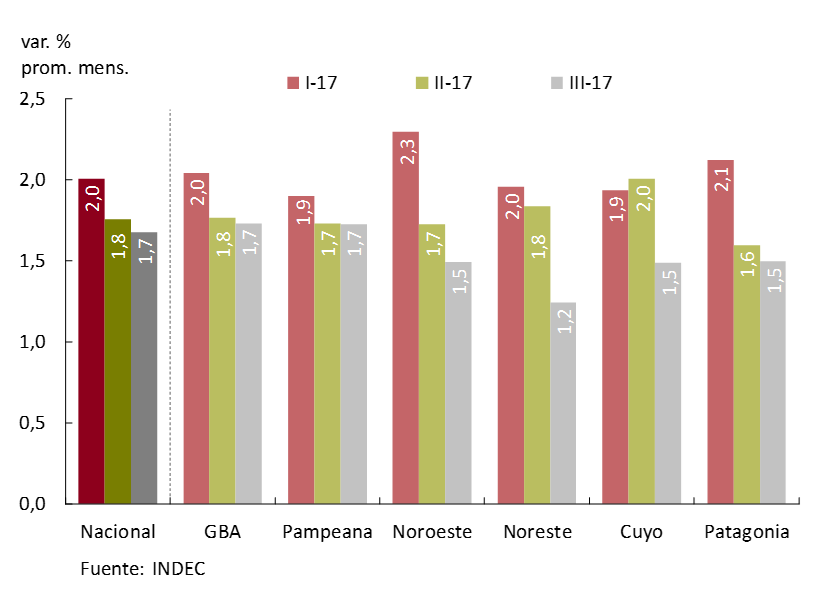
Graph 1 | National and regional inflation rates. Core

Although core inflation is falling, it is not doing so at the desired speed. For this reason, since the beginning of the second quarter of the year, the Central Bank identified the persistence of core inflation as a challenge to the ongoing disinflation process. In line with this diagnosis, the anti-inflationary bias of monetary policy was accentuated in the third quarter of the year.
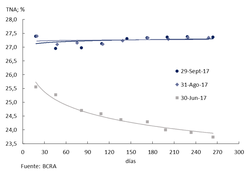
Although the rate of 7-day passes continued at 26.25%, two factors account for the greater anti-inflationary bias. First, the rise in the real ex ante interest rate that occurs when the same nominal rate is combined with a fall in expected inflation rates. Second, a reduction in the liquidity of the economy through operations of the monetary authority that were reflected in a marked change in the slope of the yield curve of the LEBACs, which occurred both from the cut-off rates determined in the tenders and also with the activity of the BCRA in the secondary market. This deliberate action has the associated benefit of lengthening the average term of the stock of liabilities, which facilitates the management of the monetary authority’s balance sheet and reduces the uncertainty associated with punctual maturities. The transmission to market rates was in accordance with the anti-inflationary sense sought by monetary policy.
Graph 2 | LEBAC Secondary Market Yield Curve (Month-End Data)
The rate of expansion of economic activity in the third quarter was around 4% annualized, and GDP thus exceeds its previous peak. Unlike other recent cycles, the current expansionary phase is reached with a greater intensity of investment. The reforms introduced since December 2015 have led to a reduction in the cost of capital and the reduction in uncertainty broadens the planning horizon of households and firms. These elements augur a broader expansive cycle than the previous ones. The REM data confirm the expectation that during 2018 the economy will continue on this path of growth, breaking with a period of six consecutive years in which a year of expansion was followed by one of contraction.
Combining the projected results for activity and inflation, the 2017-2018 biennium is expected to be the first since 2003-2004 in which there will be simultaneously a decrease in the inflation rate and an increase in the level of activity.
2. International context
The international context impacts Argentina mainly through three channels. Firstly, the level of global activity has a direct impact on our foreign trade and on potential foreign investment flows. Second, the conditions of international credit markets influence the cost of sovereign borrowing and the cost of financing private projects. Finally, the terms of trade impact our foreign trade, affecting wealth and the incentives to produce, consume and invest.
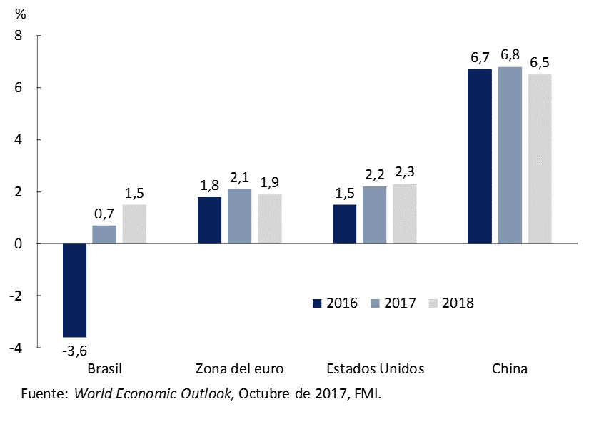
Global economic activity continued to improve in recent months, both in advanced and emerging countries, in a context of lower volatility in financial markets. Among Argentina’s main trading partners, there is an improvement in the level of activity. Projections for the remainder of 2017 and 2018 show that this dynamism in the level of activity would generally be maintained, both globally and in the case of our trading partners (see Figure 2.1). The latter would have a positive impact on Argentina (see Section 3.2.2.). In addition, credit conditions for Argentina continue to be favorable, both for the public sector and for companies. Meanwhile, the prices of Argentina’s main export commodities remained stable in recent months, and the multilateral real exchange rate depreciated 9% in the third quarter of the year.
The main risk that could alter this scenario is related to the impact on financial markets that potential protectionist measures related to Brexit would have, or the lack of agreement on the revision of NAFTA. In addition, geopolitical tensions on the Korean peninsula (and to a lesser extent on the Iberian peninsula) could also affect this scenario.
Figure 2.1 | Growth of Argentina’s main trading partners
2.1 The recovery of the activity of our business partners is highlighted
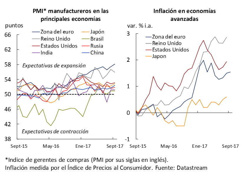
The leading indicators of activity available for the main economies show in all cases levels consistent with an expansion of economic activity, in most cases better than those observed in the previous IPOM. On the other hand, lower inflation in the United States and the Eurozone, linked in part to the fall in oil prices, reversed after the increase in oil prices in recent months (it increased 20% from the previous low in mid-June). Thus, the inflation rate in advanced economies has had an upward trend in recent months, approaching the monetary authorities’target 1 in the two aforementioned economies, and exceeding it by almost 1 p.p. in the case of the United Kingdom (see Figure 2.2).
Figure 2.2 | Leading indicators of manufacturing activity and inflation
With respect to Brazil, Argentina’s main trading partner2 and a determinant of the region’s economic performance, its level of activity continues to show signs of recovery, reinforcing the trend indicated in the IPOM of July 2017. In particular, GDP registered the second consecutive increase in the second quarter (0.2% compared to the previous quarter, without seasonality), while the Economic Activity Index, prepared by the Central Bank of Brazil (BCB, see Figure 2.3), showed the highest growth in more than three years in July (1.5% without seasonality). In turn, in July, the Industrial Production Index registered the third consecutive growth rate (for the first time since the end of 2013) with an increase of 2.5% year-on-year.
The IMF forecasts an increase in Brazilian GDP of 0.7% and 1.5% for 2017 and 2018, respectively3 (a change of 0.5 and -0.2 p.p. compared to last April). If these forecasts materialize, they would imply a favorable impact on bilateral trade, in a context where the bilateral exchange rate (Argentine peso against the Brazilian real) accumulated a depreciation of 14% in 2017 (7.2% in real terms). The higher growth of Brazilian GDP forecast for 2018 would contribute only 0.14 p.p. of growth to Argentine GDP in 2018. 4
Figure 2.3 | Brazil. Macroeconomic indicators
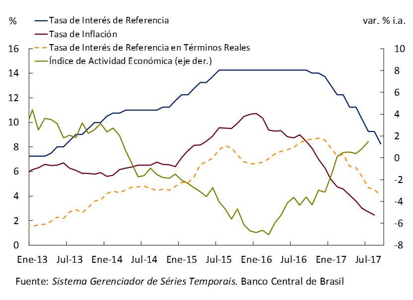
This evolution of the level of Brazilian activity took place in a context of marked disinflation, allowing an aggressive reduction of the monetary policy interest rate (the target on the Selic rate). This is how the latter went on to stand at 8.25%, 200 basis points less than its value of June 2017. According to the Focus survey, further reductions in the monetary policy rate are expected before the end of the year, by an additional 125 basis points. In addition, since inflation expectations were reduced less than the monetary policy rate, the real interest rate also suffered significant reductions.
In the euro area, the second destination for Argentine exports, both the growth data for the second quarter and the leading indicators (see Figure 2.2), and the projections for the remainder of the year and 2018 continue to show a consolidation of the recovery. Seasonally adjusted GDP grew by 0.6% in the second quarter compared to the previous quarter. In year-on-year terms, the level of activity increased by 2.1%, the highest rate of change since the first quarter of 2011. For its part, the Purchasing Managers’ Index (PMI) of the manufacturing sector (leading indicator of industrial production) registered in September the highest value since 2011. The IMF’s latest projections show that growth of 2.1% and 1.9% is expected for 2017 and 2018, (0.4 p.p. and 0.3 p.p. more than the previous projection, respectively).
In this context, the ECB decided to keep its monetary policy interest rate at the historic low of 0%, with an inflation rate below the target (less than 2%). By the end of October, the ECB is expected to start discussing possible reductions to its asset purchase program.
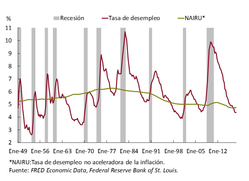
The growth of the economy of the United States, the third destination for Argentine exports, accelerated to 3.1% (annualized) in the second quarter, above market projections, in a context of lower job creation in recent months. Despite this, the unemployment rate (4.4% in August) is almost at its lowest since early 2001, and below the estimated values of the non-accelerating inflation rate (NAIRU, see Figure 2.4). Given that the labor factor would have reduced growth potential, and that according to some authors5 both the rate of return on capital and total factor productivity are at historically low values, the growth rate of the United States could be lower in the coming years than in the recent past.
In turn, the IMF again lowered (after the previous reduction in April) the growth projections for 2017 and 2018, to 2.2% and 2.3% (a decrease of 0.1 and 0.2 p.p., respectively), mainly due to the lack of fiscal stimulus measures.
In addition, the Fed’s FOMC announced at its September meeting that it will begin its balance sheet normalization program in October,6 which in practice implies a less expansionary bias of monetary policy. For the remainder of 2017, a new increase in its benchmark interest rate is expected, which would end the year in the range of 1.25-1.5%.
Figure 2.4 | United States. Unemployment indicators
China, the main destination for Argentina’s primary product exports, is expected to end 2017 with year-on-year GDP growth of 6.8% (0.2 p.p. more than the previous projection). The dynamism of the economy during the first half of the year stands out, partially linked to the postponement of reforms to correct the fiscal deficit, which reached 3.6% of GDP in 2016, and to the high rate of public investment. An increase in imports was also evident in recent months, which would end the year with a year-on-year growth of 11.2%, partly driven by an appreciation of the yuan of 5%. Finally, for 2018, a lower GDP growth rate of around 6.5% is expected.
2.2 Favorable credit conditions continue for Argentina
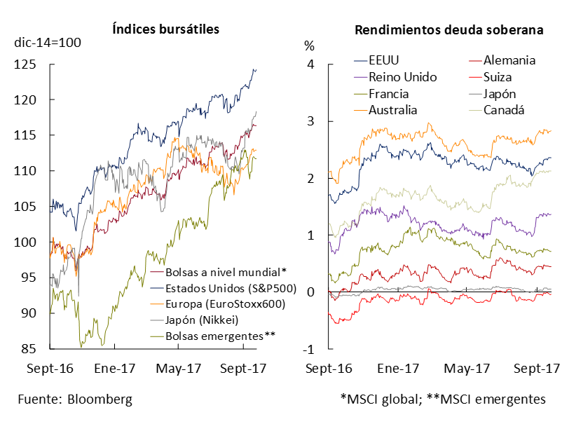
International financial markets continued to generally have a period of improvement and lower volatility for both equity and fixed income assets, and in advanced and emerging economies. The Fed’s announcement in late September that it will begin tapering its asset purchase program from October, along with the possibility that the ECB will soon start discussing this issue as well, had a limited impact on markets, especially sovereign debt markets (see Figure 2.5).
Figure 2.5 | stock indices and 10-year sovereign bond yields
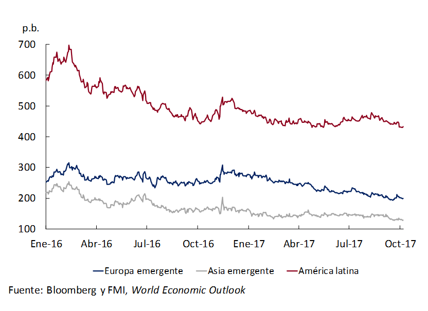
Over the past few months, sovereign risk premiums have continued their downward trend, remaining almost unchanged between peaks in Latin America (see Figure 2.6).
Figure 2.6 | Emerging. Sovereign risk premiums
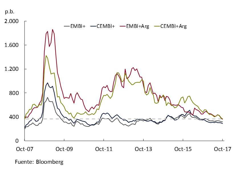
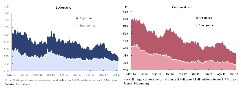
Debt issuances from emerging countries increased by 37% so far in 2017 compared to the same period in 2016, with the corporate sector having both greater participation and greater dynamism. For Argentina, credit conditions improved even more than for the rest of the emerging countries, placing the Argentine country risk at around 360 bps for the EMBI+ Argentina index, and at 368 bps for the CEMBI+ Argentina, in both cases the lowest value in the last ten years (see Figure 2.7). The corporate risk spread with respect to other emerging markets was also reduced (see Section 3.3). Therefore, the public sector and Argentine companies are financing themselves at lower interest rates in international markets.
Figure 2.7 | Sovereign and corporate debt risk indicators
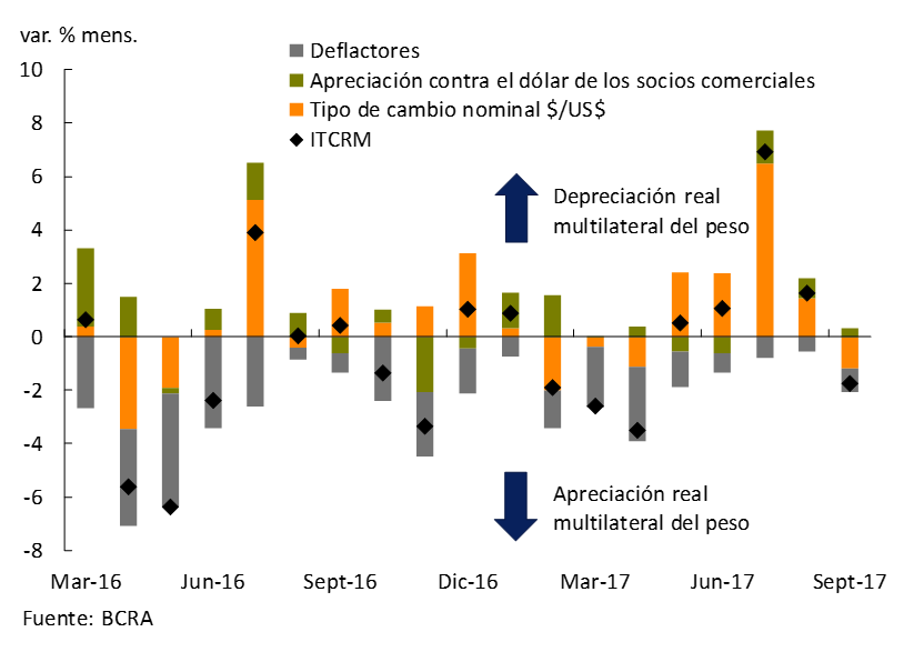
The Multilateral Real Exchange Rate Index (ITCRM) depreciated 8.7% in the quarter, driven both by the depreciation of the peso against the dollar by 9.9%, and by the appreciation of the currencies of our trading partners (also against the dollar) by 2.7%; and partly offset (3.9%) by higher Argentine inflation compared to that of our trading partners. The largest nominal (and real) depreciations of the peso were observed in July and August (see Figure 2.8).
Figure 2.8 | ITCRM variation by component
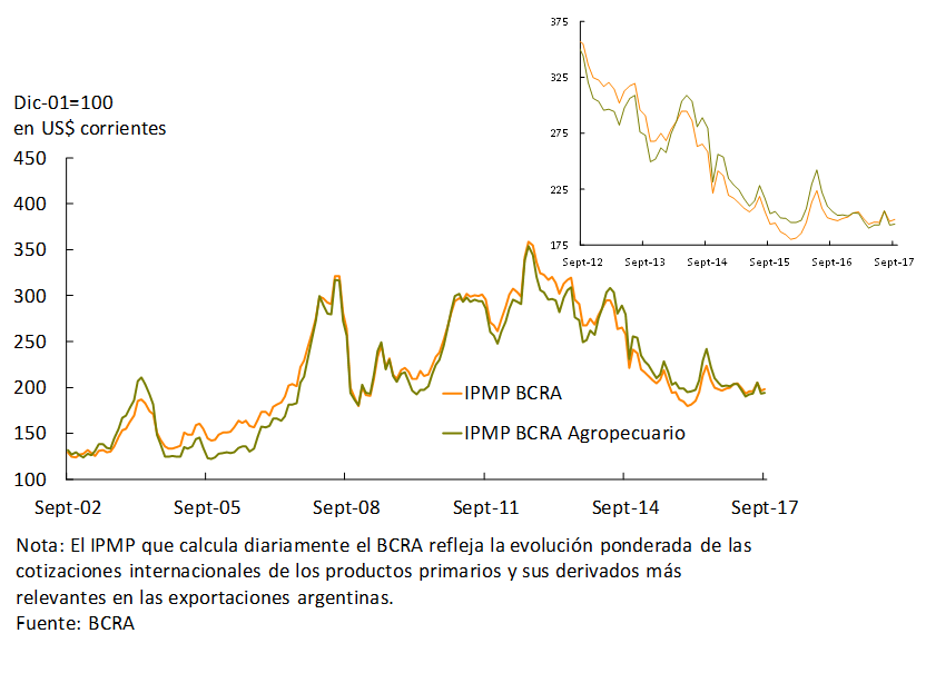
The Commodity Price Index (BCRA MPPI) – which reflects the evolution of Argentina’s main export commodities, with a marked influence on the Argentine economic cycle – remained relatively stable in recent months (0.09% year-on-year variation). In the case of the agricultural BCRA MPPI, the downward trend of recent months continued (-20% compared to June 2016), although during 2017 it remained stable beyond some occasional volatility (see Figure 2.9).
Figure 2.9 | International commodity prices
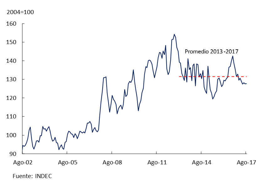
Finally, the terms of trade (quotient between the prices of Argentine exports and imports)7 remained relatively stable in recent months around the 2013-2017 average (with data up to August; see Figure 2.10).
Figure 2.10 | Terms of exchange
In summary, it is expected that a sustained growth rate will be maintained globally in the coming months, especially in our main trading partners, which would have a favorable impact on the demand for Argentine exports. In addition, conditions of abundant liquidity continue to exist for emerging countries, despite the tightening of the Fed’s monetary policy that would not have a significant impact on financing costs. Therefore, credit conditions for Argentina are expected to remain favorable. The main risks would be linked to the impact on financial markets of protectionist measures and geopolitical tensions on the Korean peninsula (and to a lesser extent on the Iberian peninsula).
3. Economic activity
The expansion of the last twelve months, at a rate of around 4% annualized, allowed GDP to exceed the peak of 2015 in the third quarter of this year. The new economic configuration, together with actions aimed at strengthening macroeconomic stability, led to a reduction in the cost of capital and extended the planning horizon of companies and families. The current phase of growth is characterized by increased investment intensity and is accompanied by widespread increases in employment at the sectoral level. Going forward, these trends will strengthen, allowing the stagnation of the economy of the last six years to be broken.
Figure 3.1 | Level of economic activity
3.1 Growth of the economy is consolidated
The structural reforms implemented since 2016, as well as the fiscal and monetary order of the economy, are bearing fruit in terms of economic growth. This is taking place in a favorable international context in which the economies of our trading partners are growing (see Box) and in which there is abundant liquidity in international financial markets. As anticipated in the previous IPOM, the evolution of the Argentine economy continued to show features typically observed in the growth cycles of Latin American countries. During the second quarter of the year, the components of domestic expenditure (consumption and investment) grew above income (GDP), so net exports were reduced. The greater dynamism of domestic spending led to a recovery in the relative price between non-tradable and tradable products.
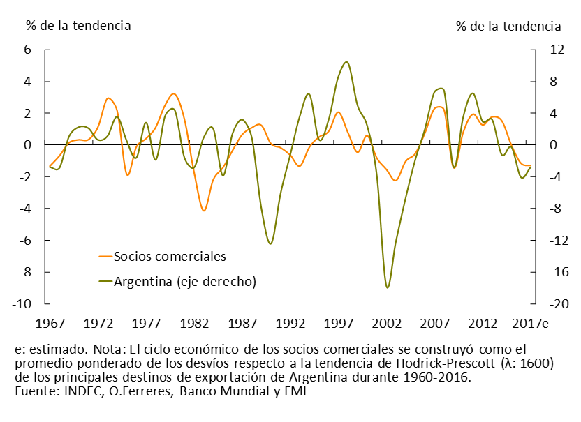
Box. Synchrony of cycles of the Argentine economy and its trading partners
Since the mid-twentieth century, it has been observed that Argentina’s economic cycle was mostly synchronized with those of its main export destinations. 8 In fact, the correlation between the two series is 0.46 during the period 1966-2016. In addition, historical evidence shows that the Argentine cycle has a higher degree of volatility: Argentina’s standard cycle deviation is 3.5 times higher than that of the cycle of its main trading partners as a whole (see Figure 3.2).
The periods in which divergences were observed coincided with idiosyncratic disturbances that altered local activity. Among them are the Falklands War and the return to democracy in the period 1982-1983, hyperinflation in 1989-1990, the beginning and end of the convertibility regime and, more recently, the validity of the exchange clamp between 2012 and 2015 – which introduced distortions into the economy with their respective cost in terms of efficiency. After these disturbances, the Argentine economic cycle returned to its usual synchrony.
Figure 3.2 | Economic cycles of Argentina and its trading partners. Deviations from its trend
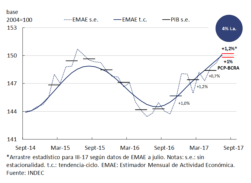
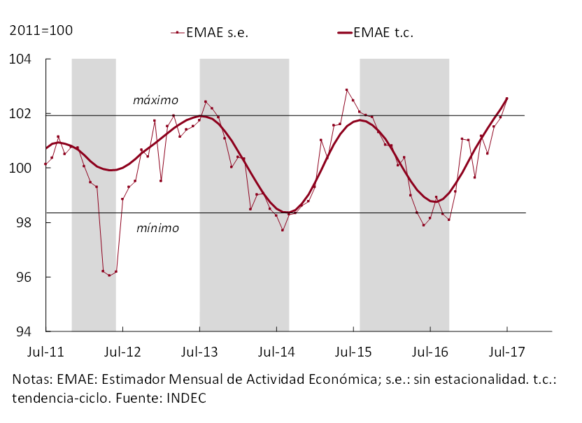
During the second quarter of 2017, GDP growth was 2.7% y.o.y. (0.7% s.e.), expanding at an annualized rate of 3.8% in the first half of the year. In July, the EMAE grew 0.7% s.e., leaving a statistical drag of 1.2% s.e. for the third quarter (see Figure 3.1).
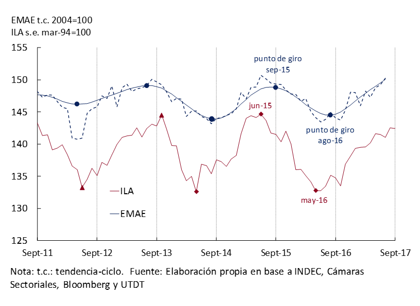
By the third quarter, GDP surpassed the previous peak of 2015, completing a year of continuous growth at an average annualized rate of 4%. The latest Contemporary GDP Prediction of the BCRA (PCP-BCRA) indicates a quarterly increase of 0.95% s.e. while the forecast of the analysts of the Market Expectations Survey (REM) is 1.2% s.e. The coincident indicator prepared by the Undersecretariat of Macroeconomic Programming estimates a growth of 1.3% s.e. The data for September from the Leading Indicator of Activity (ILA) prepared by the BCRA, which anticipates the turning points of the EMAE, indicate that the economy will continue to expand during the last quarter of the year (see Figure 3.3).
Figure 3.3 | Leading Activity Indicator
3.2 The current macroeconomic configuration breaks with the previous stagnation
The last six years have been characterized by high output volatility, around a stagnant trend9 (see Figure 3.4). This behavior evidenced limitations in the determinants of supply that operated until the end of 2015. Macroeconomic imbalances, relative price distortions, and exchange rate constraints led to significant declines in the investment rate, which led to a stagnation of potential GDP and productivity during that period. Between July 2011 and July 2017, activity exhibited an average annual growth of 0.4%, lower both than population growth and the rise in total urban employment (1.1%), generating a continuous deterioration in per capita income.
Figure 3.4 | Evolution of economic activity in the last 6 years
The pursuit of fiscal and inflation targets aimed at strengthening the macroeconomic environment, the resolution of the conflict with the holdouts, the normalization of the exchange rate, the elimination of distortions and taxes on foreign trade, among other measures, extended the planning horizon of agents and reduced the cost of capital. The corporate risk differential with respect to other emerging markets is below 100 bps, at the lowest levels since 2010 (see Figure 3.5). This new macroeconomic configuration together with the expected improvements in infrastructure also increased the marginal return on expected capital. In this context, the expansion of the economy of around 4% annualized during 2017 with increases in employment and the growing contribution of investment, will make it possible to overcome the stagnation of recent years (see subsections 3.2.1 and 3.2.3).
Figure 3.5 | Cost of financing
3.2.1 Investment takes on a leading role in the current stage
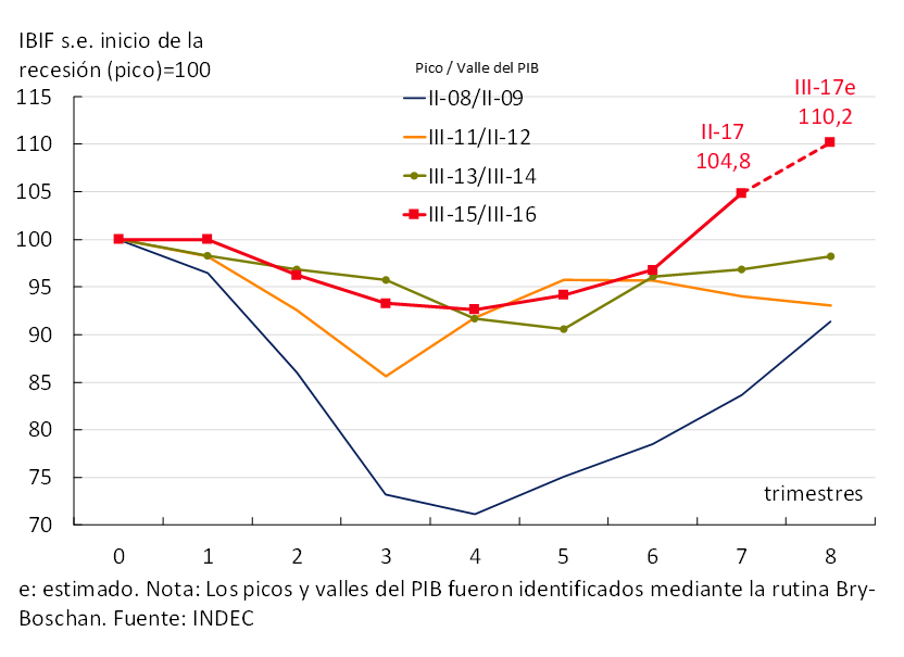
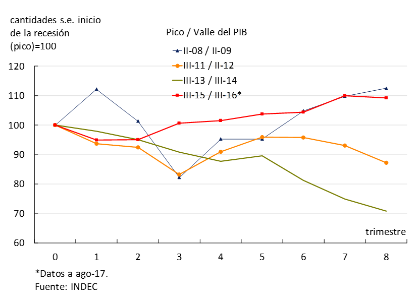
In line with what was anticipated in the previous IPOM, gross domestic fixed investment (GDI) increased strongly in the second quarter (8.3% s.e., the highest growth since the second quarter of 2010). This performance made it possible to exceed the level corresponding to the beginning of the last recession (III-15), with this recovery in investment being the fastest and most intense of the last four, including that of 2009/2010 (see Figure 3.6). For the third quarter, this trend is expected to continue, according to the Coincident Investment Index prepared by the Ministry of Finance (5.1% s.e.).
Figure 3.6 | Investment. Latest business cycles compared
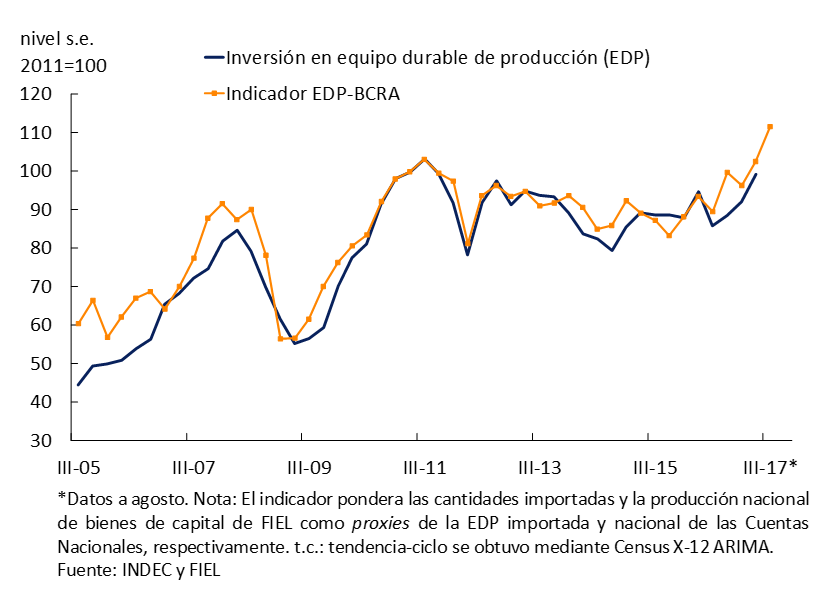
The growth in investment was highlighted by a sharp increase in expenditure on durable production equipment (PDE)10, which is a distinctive feature of the current recovery compared to previous ones. The increase in investment in EDP during the second quarter was both domestic (7.6% s.e.) and imported (7.8% s.e.). In July and August, FIEL’s index of domestic equipment remained at a high level. In the same period, the quantities imported of capital goods reached an all-time high (+15.4% average s.e.), highlighting the increase in foreign purchases of machinery and equipment. This dynamism was reflected in the EDP-BCRA indicator, which anticipates significant growth in investment in EDP during the third quarter (see Figure 3.7).
Figure 3.7 | Investment in durable production equipment
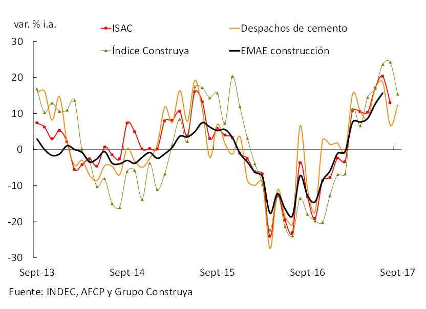
Construction continued to grow during the third quarter driven by private and public works, recovering the maximum level reached in 2015. Cement shipments to the domestic market grew 6.1% s.e. between July and September, while the Construya index, which mainly captures items associated with the completion of private works, expanded 9.6% s.e. (see Figure 3.8).
Figure 3.8 | Evolution of construction
3.2.2 Domestic expenditure and net exports showed traits typically observed in the expansion phases
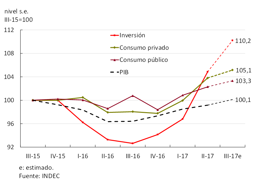
In addition to investment, private consumption accelerated its growth rate (3.8% s.e.), contributing 2.8 (p.p.) to the change in GDP11 and exceeded the pre-recession peak (see Figure 3.9).
Figure 3.9 | Composition of aggregate domestic expenditure in the current recovery
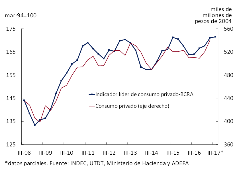
Various indicators show that this behavior was maintained during the third quarter, including the quarterly growth of real gross VAT (2.9% s.e.) and the increase in imports of consumer goods (15% s.e.) in the July-August two-month period. Going forward, the Leading Indicator of Private Consumption – BCRA12 anticipates that the positive trend will continue (see Figure 3.10). Private consumption grew underpinned by the continued improvement in real household wages, the expansion of employment, credit and public spending on social benefits, in a context of rising consumer confidence. During the third quarter, consumer credit (personal loans and credit cards) grew 4.1% s.e. in real terms, and social security benefits and social plans rose 4.5% s.e. between July and August.
Figure 3.10 | Evolution of private consumption
As is foreseeable in an expansive phase of the economic cycle, the greater strengthening of investment and private consumption compared to Income13 led to net exports being negative and would continue to be so in the third quarter. Exports of goods and services fell 7.1% s.e. in the second quarter,14 as anticipated in July’s IPOM and are estimated to recover during the third quarter, according to foreign trade data for July and August. Imports grew 4.2% s.e. in the second quarter with an outstanding performance of capital goods, a trend that continued between July and August.
Figure 3.11 | Quantities exported and business cycle of trading partners
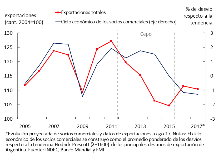
During the period of the clamp, total exports exhibited an unusual decoupling from the cycle of trading partners, a behavior that normalized after the macroeconomic reconfiguration at the end of 2015 (see Figure 3.11). Since 2016, exports of Manufactures of Industrial Origin (MOI) have had one of the best performances throughout the economic cycle compared to other recent episodes of decline and recovery (see Figure 3.12).
Figure 3.12 | Exports of manufactures of industrial origin. Latest Cycles Compared
3.2.3 Growth in activity and employment was spread among the productive sectors
The growth of the economy was highly disseminated at the sectoral level. Among the most dynamic activities in the last year are fishing, construction, financial intermediation, agriculture, and transport and communications. Construction continues to grow based on private and public works. Financial intermediation was driven by the drop in expected inflation that allows the credit horizon to be extended, the implementation of measures aimed at facilitating the operation of the banking system15 and the strong demand for credit in UVAs, which is growing at a rate of 50% per year. The agricultural sector continues to respond positively to the elimination/reduction of export duties and exchange rate normalization (see Figure 3.13).
Figure 3.13 | Economic growth by productive sector. Second quarter 2017
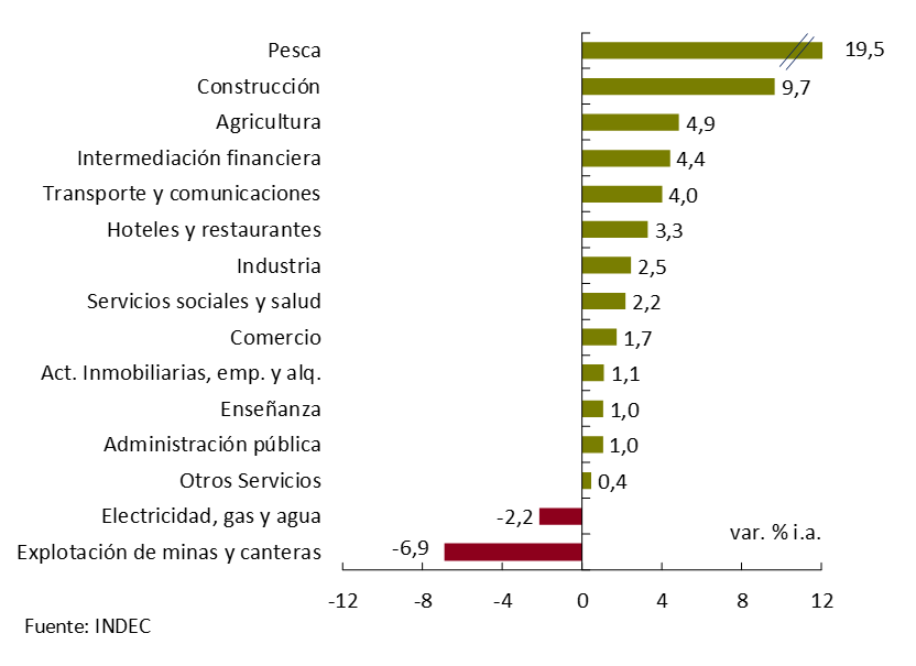
The only sectors that contracted – representing 4.6% of GDP – were electricity, gas and water, and mining and quarrying. In the first case, higher temperatures compared to the previous year together with the removal of subsidies reduced residential demand. In the second, the current international oil prices were not profitable to break the declining trend in production since 1998, while the reduction in mining exploration in recent years had a negative impact on the sector’s activity.
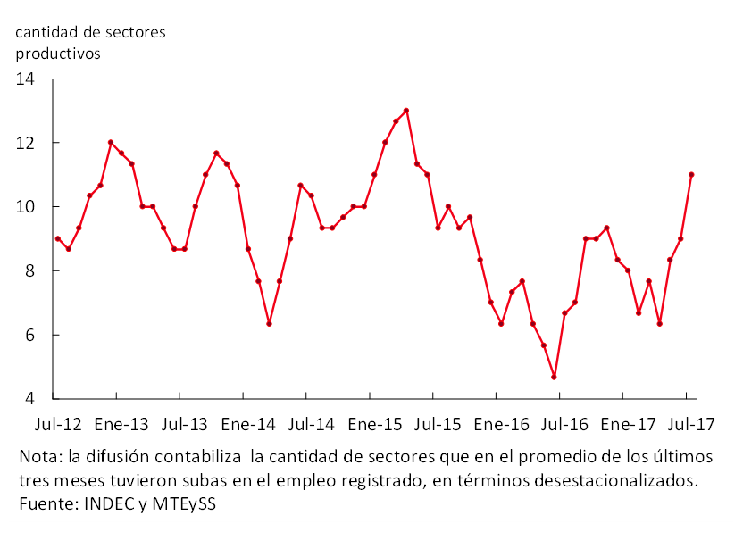
As economic activity consolidates its growth, the number of productive sectors that increase their number of registered employment increases. The sectoral diffusion of employment generation in the private sector continued its upward trend in the second quarter and would have remained at high levels during the third quarter (see Figure 3.14).
Figure 3.14 | Diffusion of wage employment growth in the private sector
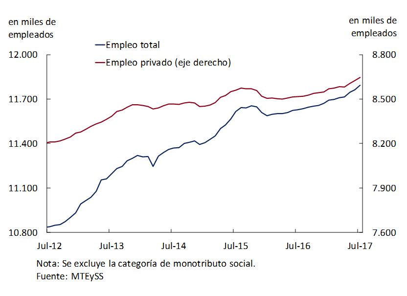
Registered employment continued with the positive trend that began a year ago, exceeding the previous maximum level. In the year it accumulated an increase of 1% s.e. (see Figure 3.15), highlighting in the last twelve months the greater dynamism of the private sector registered (1.5% y.o.y.) compared to that of the public sector (1.1% y.o.y.).
Figure 3.15 | Evolution of registered employment without seasonality
In terms of employment rates and total unemployment, there were no significant variations in the last year. 16 The recovery in job creation was slightly lower than population growth, so the employment rate remained practically unchanged.
3.3 Outlook: Argentina’s economy expected to return to sustained growth
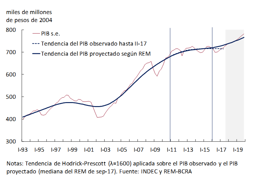
As a result of the new macroeconomic configuration, the BCRA expects the economy to consolidate its growth process, leaving behind the stage of trend stagnation. This view is in line with the estimates included in the 2018 National Budget Bill, which contemplates growth of 3% in 2017 and 3.5% for 2018-2019 and is shared by the participants of the Market Expectations Survey (REM) who projected that the economy will continue to expand annually by 2.8%, 3% and 3.2% between 2017 and 2019. These prospects implicitly contain a break since 2016 in the medium-term trend of GDP growth17 (see Figure 3.16.).
Figure 3.16 | GDP. Medium-term trend projected according to REM
Greater macroeconomic certainty together with the favorable prospects for economic growth and productivity, together with the fall in the cost of capital, will continue to be decisive in boosting investment. The development of infrastructure will be a key factor in boosting the productivity of the economy. 18 The Public-Private Partnership Law (PPP), the productivity agreement for the exploitation of Vaca Muerta19 and the award of alternative energy production projects within the framework of RenovAR20, will allow the development of infrastructure, technology and energy projects, among others. According to data from the Chief of Cabinets of Ministers, investment in infrastructure will go from 269,417 million pesos (2.6% of GDP) in 2017 to 436,313 million pesos in 2018 (3.5% of GDP), increasing 50% in real terms (see Section 3 / Public-private participation).
The great potential of mortgage loans in UVAs in a context of low level of indebtedness of households and companies21 (mortgage credit is 0.9% of GDP in Argentina vs. 10% of GDP on average in other emerging economies), favor the development of real estate activities and construction. Empirical evidence suggests that access to housing finance can continue to be facilitated through a robust legal framework and a stable macroeconomic environment. 22
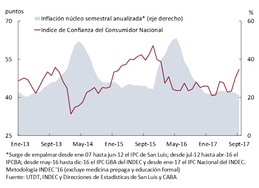
The better prospects of trading partners will boost external sales of manufactures of industrial origin, which together with a harvest around its historical highs will lead to an expansion of exports. Consumption will continue to be driven by employment growth and lower inflation, which strengthens the purchasing power of wages and has a positive impact on consumer confidence (see Figure 3.17).
Figure 3.17 | Consumer Confidence Index and Inflation
From the point of view of supply, the use of productive factors is below the level that would cause inflationary pressures, a dynamic that will continue to be monitored by the BCRA.
4. Pricing
In the third quarter, inflation showed a slight slowdown compared to previous quarters, averaging a monthly increase of 1.7%. The core component increased at a monthly rate of 1.6%, 0.1 p.p. less than the previous quarter. Core inflation was at the lowest levels in recent years, although it continues to be above the level sought by the monetary authority, showing some persistence. During the third quarter, inflation was 22.7% YoY, 1.7 p.p. lower than in the previous quarter. Inflation expectations indicate that the disinflation process will continue in the medium term. The forecasts of the analysts participating in the Market Expectations Survey (REM) anticipate a gradual moderation. Although market forecasts are still above the inflation targets set by the Central Bank, they are lower than those observed in the last eight years.
Figure 4.1 | CPI. Headline
4.1 Inflation continued to decelerate.
In the third quarter of the year, the process of deceleration of retail prices continued, although with rates higher than those sought by the Central Bank for this period. CPI23 registered an average variation of 1.7% (22.1% annualized), 0.1 p.p. lower than that of the second quarter (see Figure 4.1). Coreinflation 24 showed a similar dynamic to that of the general level, increasing at a monthly rate of 1.6% in the third quarter (0.1 p.p. below the previous period; see Figure 4.2).
In the first nine months of the year, retail prices accumulated an increase of 17.6% in the general level and 16.1% in their core component. As expected, the year-on-year variation of the CPI increased in August and September of this year, due to the effect of a lower base of comparison as a result of the temporary suspension of the tariff increase for gas service by network during these months in 2016. Meanwhile, the core measurement, which excludes regulated ones, maintained a downward trajectory in its year-on-year comparison.
Figure 4.2 | IPC Core
This lower dynamism of the general level occurred in a context in which the process of updating the relative prices of regulated items continued. This group accumulated a 23.2% increase so far this year, placing it above core inflation. Seasonal goods and services exhibited an accumulated annual increase of 16.2%, in line with the rise in core inflation.
Figure 4.3 | Core Inflation
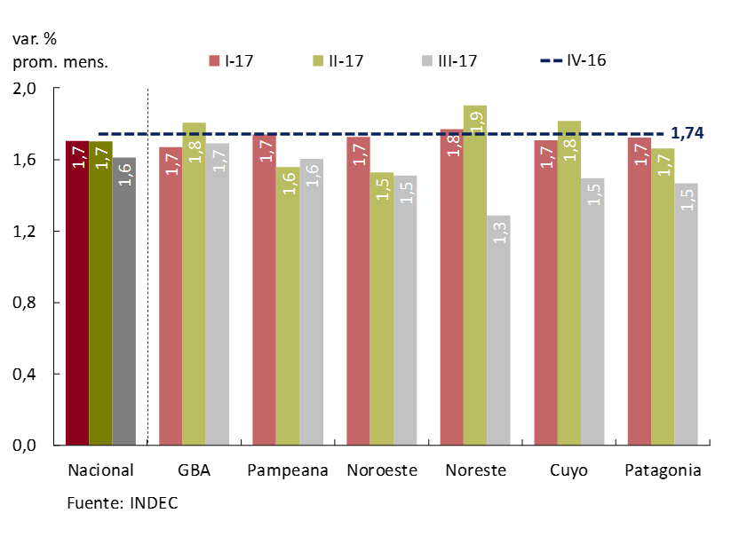
Core inflation maintained some persistence in its monthly growth rate at the national level. This dynamic mainly reflects what happened in the GBA and the Pampas region, which represent almost 80% of the index. The rest of the regions showed a slowdown that is more marked in the Northeast region. The measurement of the City of Buenos Aires and other core inflation indicators prepared by the BCRA24 based on disaggregated information from that index, also maintain a stable growth rate in relation to recent quarters. Despite the persistence of core inflation, it is at the lowest values in recent years (see Figure 4.3). Data from the first days of October from the PriceStats high-frequency index indicate that inflation would show a slowdown (1.2% variation 30 moving days).
Figure 4.4 | Core inflation trend by Private Goods and Services – City of Buenos Aires.
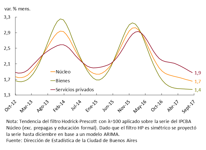
To analyze the behavior of core inflation by goods and services, the CPI of the City of Buenos Aires was used, since there is not enough disaggregated information on the CPI prepared by INDEC. 25 During the third quarter of the year, the prices of goods in the core component continued to grow at a lower rate than that of private services. 26 Inflation in goods remained at a rate similar to that of the first half of the year, while inflation in private services continued to decelerate (see Figure 4.4). This dynamics of services is consistent with the rates of increase in nominal wages, in a context of growth in economic activity (see subsection 4.2).
The adoption of an inflation targeting regime with floating exchange rates sought to achieve the disinflation of the economy without the need to use the exchange rate as a nominal anchor (see Monetary Policy section). The correlation between the nominal exchange rate and core inflation since the change of regime was negative (-0.33), while between 2011 and 2015 the coefficient was positive (0.43). This decoupling between the variables can also be verified through the relative volatility between changes in the nominal exchange rate and inflation, a relationship that has increased significantly since the change of regime (see Figure 4.5).
Figure 4.5 | Prices and Nominal Exchange Rate
Wholesale prices registered an average monthly growth rate of 1.8% during the quarter. In year-on-year terms, these prices registered a growth rate of 16.3%, standing 7.5 p.p. below the year-on-year rate of increase in consumer prices (see Figure 4.6).
Figure 4.6 | Wholesale and retail prices
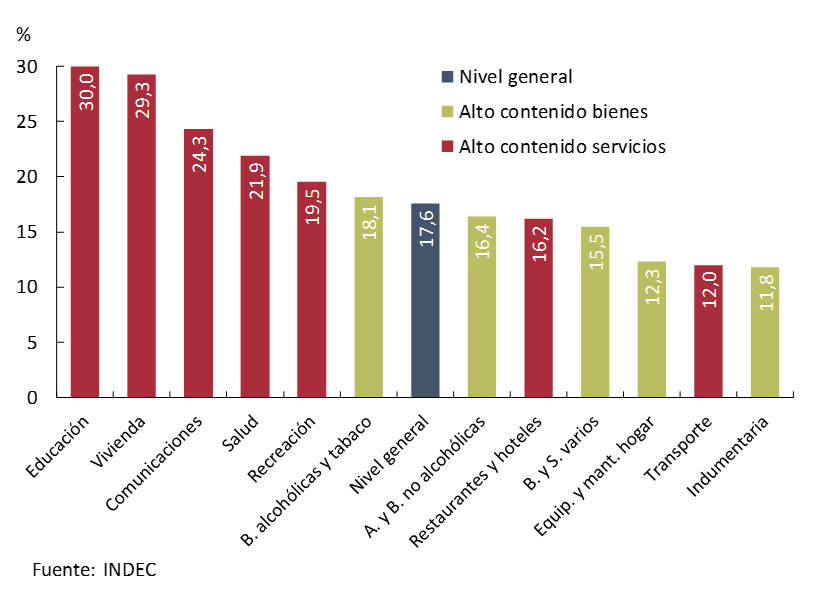
Disaggregating the CPI by divisions, it can be seen that in cumulative terms, the divisions associated with total services (regulated and non-regulated) are the ones that showed the highest increases. In the case of regulated ones, it is explained by the process of updating tariffs, after several years in which they remained unchanged. Divisions with a higher share of goods helped to take pressure off inflation. Those that benefited from a context of greater trade liberalization stood out, such as household equipment and maintenance, a division that includes the evolution of prices of household appliances and electronics (see Figure 4.7).
Figure 4.7 | National CPI. Opening by divisions
4.2 Nominal wages moderated their growth rate
In the third quarter, nominal wages would have increased at a rate higher than inflation. A slowdown in the pace of growth in labor costs is expected for the latter part of the year, given the structuring of wage agreements (see Figure 4.8).
Figure 4.8 | Salaried private sector remuneration (mobile avg. 3 months)
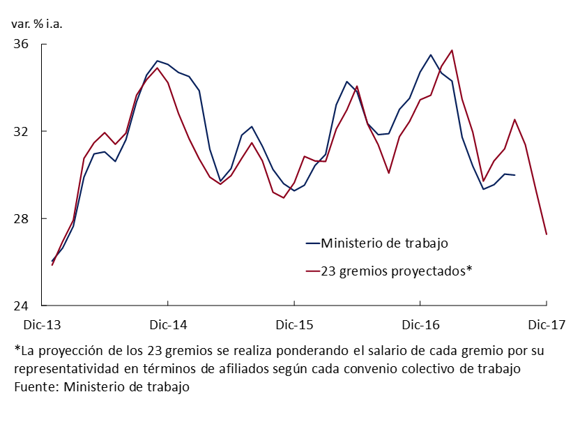
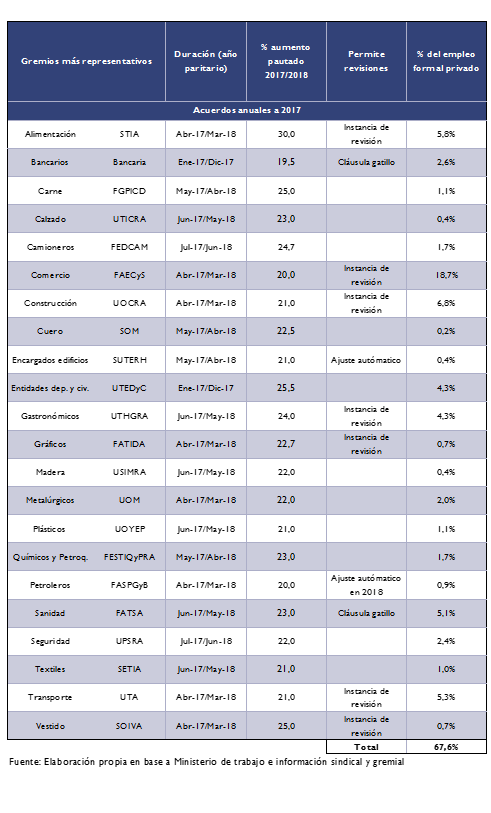
Most of the adjustment clauses included in the collective bargaining agreements would not enter into force, since inflation would be below the agreed wage increases (see Table 4.1). If our nominal wage forecasts are met, the year would end with an average real wage increase of approximately 4%.
Table 4.1 | Collective Agreements
4.3 Disinflation would continue in the latter part of the year
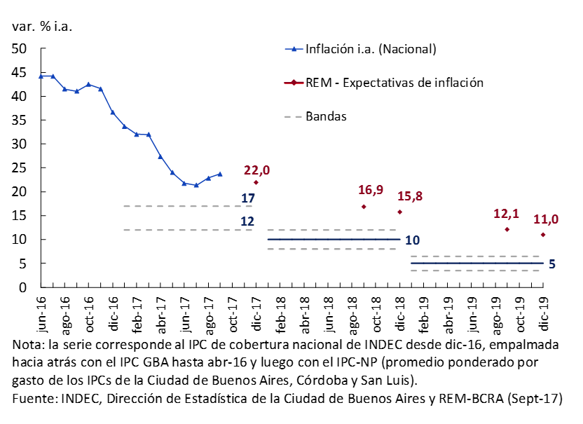
For the coming months, market analysts expect the disinflation process to continue, albeit gradually, as reflected in the expectations captured by the REM. For the last quarter of the year, they forecast an average monthly inflation rate of 1.4% (18% annualized), lower than that recorded in the first part of the year. In year-on-year terms, expectations remained at around 22% YoY for December 2017 and at 16.9% YoY for the next twelve months (see Figure 4.9). Although market forecasts are still above the inflation targets set by the Central Bank, they are lower than those observed in the last eight years.
Figure 4.9 | Inflation targets and expectations
5. Monetary policy
The primary objective of monetary policy is to achieve low and stable inflation. To this end, the Central Bank defined a decreasing path of inflation targets: between 12% and 17% for 2017, between 10% ± 2% for 2018, and 5% ± 1.5% as of 2019; and chose the interest rate on 7-day passes as the main policy instrument.
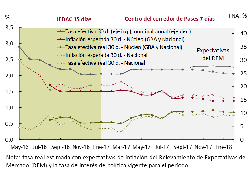
In the third quarter of the year, retail inflation continued to show a marginally downward trend, with a slight drop in the average monthly inflation rate compared to the previous quarter (see Figure 4.1). However, the inflationary process continues to show persistence in core inflation, while price increases continued above the level desired by the Central Bank, which seeks to ensure that inflation at the end of the year is consistent with the 10% ± 2% target of 2018 (see Figure 4.2). At the same time, inflation expectations increased slightly throughout the quarter, with year-on-year inflation reaching 12% in the third quarter of 2019 (see Figure 4.9). In this context, the monetary authority kept the monetary policy rate stable at 26.25% annually throughout the quarter, while the real interest rate reflected a more restrictive stance due to the downward trend shown by the expected monthly inflation rates. In addition, the Central Bank continued to operate actively in the secondary LEBAC market in order to reinforce the transfer of this more restrictive stance to the rest of the market’s interest rates, which resulted in increases in the interest rates of these instruments throughout the quarter.
Figure 5.1 | Inflation scenarios consistent with the 10% YoY target in December 2018
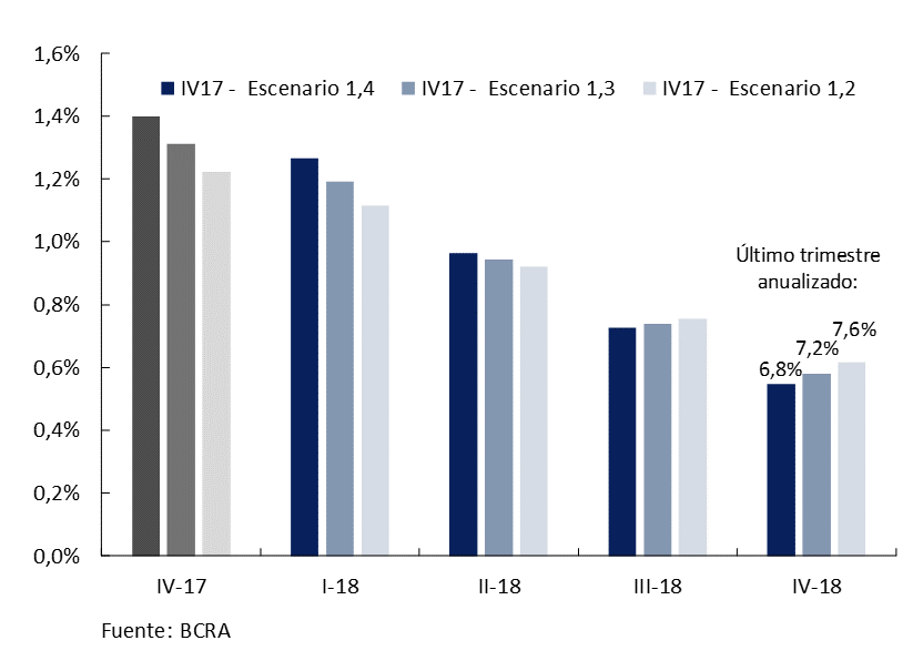
The Central Bank will continue to maintain a clear anti-inflationary bias to ensure that the disinflation process continues towards an inflation rate by the end of 2017 that is compatible with the target of 10% ± 2% for 2018. In this regard, Figure 5.1 shows different scenarios of average monthly inflation rates for the last quarter of the year with their respective trajectories during 2018 that are consistent with the 10% year-on-year target in December 2018.
5.1 The Central Bank’s monetary policy during the third quarter
The slowdown in inflation in the second half of 2016 led to a relaxation of monetary policy which, combined with increases in regulated prices, resulted in higher monthly records than those sought during the February-April period of this year. The Central Bank reacted by increasing its monetary policy rate, the center of the 7-day pass corridor, by 150 basis points, to 26.25% annually on April 11 and restricting liquidity conditions in the secondary LEBAC market, which was reflected in interest rate hikes on these instruments. These contractionary monetary policy measures resulted in a reduction in inflation thereafter.
In the third quarter of the year, retail inflation continued to show a marginally downward trend, with a slight drop in the average monthly inflation rate compared to the previous quarter (see Figure 4.1). However, the inflationary process continues to show persistence in core inflation, while price increases continued above the level desired by the Central Bank, which seeks to ensure that inflation at the end of the year is consistent with the 10% ± 2% target of 2018 (see Figure 4.2). At the same time, inflation expectations showed a slight increase throughout the quarter, marking year-on-year inflation reaching 12% in the third quarter of 2019 (see Figure 4.9). In this context, the monetary authority kept the monetary policy rate stable at 26.25% annually throughout the quarter, while the real interest rate reflected a more restrictive stance due to the downward trend shown by the expected monthly inflation rates (see Figure 5.2). 26
Figure 5.2 | Nominal and real policy interest rate
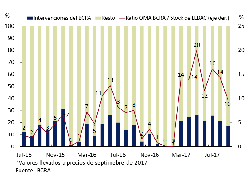
In addition to the management of the policy interest rate, the Central Bank continued to operate actively in the secondary LEBAC market in order to reinforce the transmission of this more restrictive stance to the rest of the market’s interest rates. Thus, in the third quarter the Central Bank continued to restrict the liquidity conditions of the money market by conducting operations in the secondary market of LEBAC (open market operations). Between July and September, the BCRA sold LEBAC in the secondary market for a total of VN $410.8 billion. Thus, open market operations accounted for 21% of the total operations carried out -quarterly average- in the secondary LEBAC market (see Figure 5.3).
Figure 5.3 | Central Bank interventions in the LEBAC secondary market
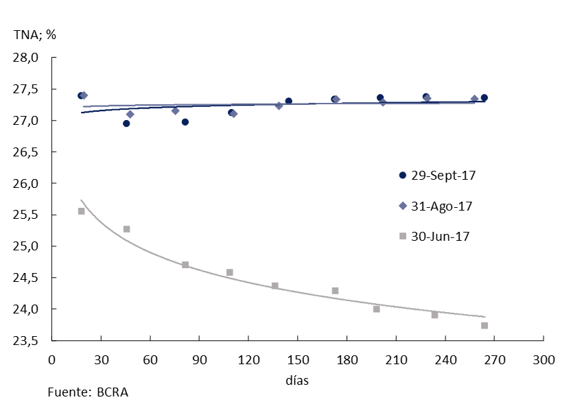
Throughout the quarter, along with tightening liquidity conditions, the monetary authority sought to modify the slope of the LEBAC yield curve. Thus, towards the end of August the yield curve observed in the secondary market began to show a flatter shape, and finally at the end of August it showed a slight positive slope (see Figure 5.4). This implied an increase of 1.7 p.p. in shorter-maturity papers and 3.6 p.p. in those with longer maturities between the end of June and the end of September. This change in the curve generated a gradual lengthening of the average term of the stock of LEBAC in circulation, which went from 43 days on average in June to 75 days on average in September.
Figure 5.4 | LEBAC Secondary Market Yield Curve (Month-End Data)
5.2 The Transmission of the Policy Interest Rate to the Other Market Interest Rates
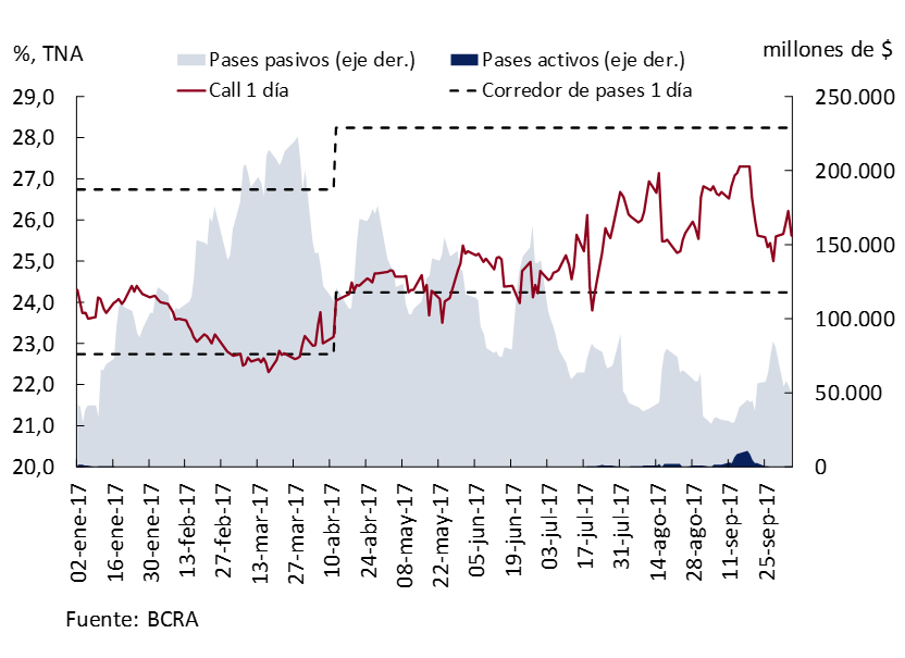
Money market interest rates continued to rise in the third quarter of the year. The restrictive liquidity conditions of the market led interest rates to leave the floor of the rate corridor to be located at levels closer to the center of said band, according to what the monetary authority sought. In this sense, the 1-day interbank call rate registered a rise of 1.7 p.p. between June and September to reach a monthly average of 26.4% annually (see Figure 5.5).
The pass corridor established by the BCRA helps to keep the volatility of interest rates in the interbank market limited: the interest rate of passive passes serves as a floor for interest rates in the interbank market, while the interest rate of active countries constitutes a ceiling. Since the change in the monetary policy instrument, the facility windows began to be used more frequently by financial institutions, especially that of active passes, whose use was previously very infrequent. Thus, as expected, the movement of rates towards the center of the corridor occurred together with a sustained reduction in the stock of passive passes throughout the quarter and with an increase in active passes, particularly in September (see Figure 5.5).
Figure 5.5 | Rate broker, 1-day call, and pass trading
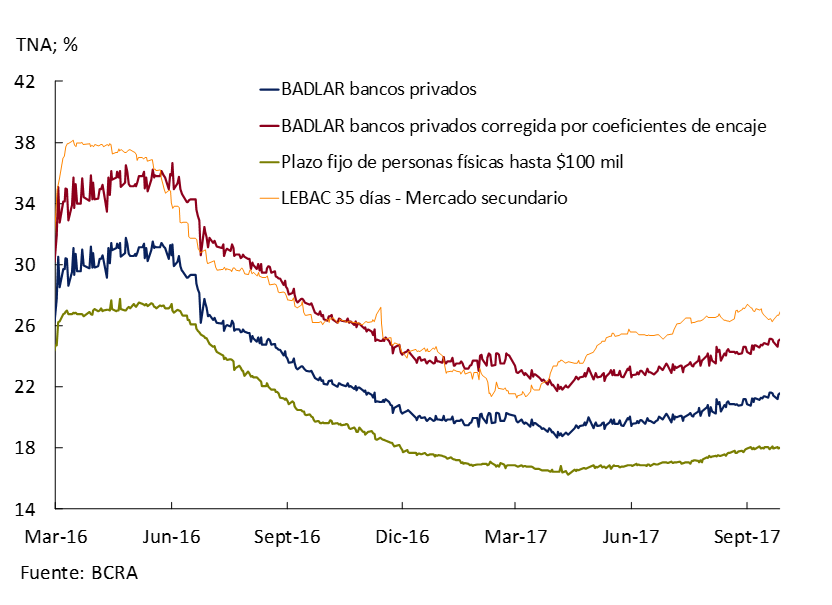
On the other hand, interest rates on deposits, which had remained relatively stable in the previous quarter, began to increase following the restrictive liquidity conditions. In the wholesale segment, the BADLAR of private banks increased 1.5 p.p. to reach a monthly average of 21.3% in September. Despite this recovery, they still lag behind when comparing the funding cost of wholesale deposits adjusted for reserve requirements with the 35-day LEBAC rate, with the spread for the quarter being 2.4 p.p. In the retail segment, the rise in interest rates on fixed-term deposits was somewhat lower, 1 p.p., to close September with a monthly average of 17.9% (see Figure 5.6).
Figure 5.6 | LEBAC rate and bank passive rates
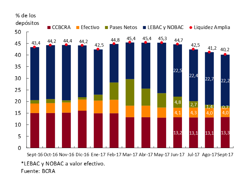
The increase in banks’ passive interest rates occurred in a context of credit expansion and a fall in the liquidity of financial institutions. In fact, the ample liquidity of the total financial system, which includes cash in banks, current account deposits in the BCRA, net passes and LEBACs, went from 44.7% in June to 40.2% in September (see Figure 5.7), with net passes explaining most of the fall.
Figure 5.7 | Liquidity ratios in pesos of financial institutions
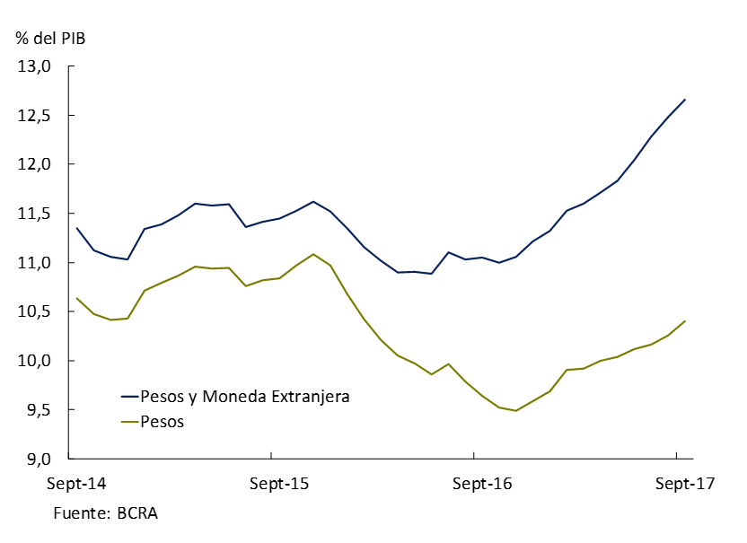
At the same time, loans in pesos to the private sector accelerated their pace of expansion in the third quarter, with an average monthly increase of 1.8% in real terms (without the effect of seasonality), while in the previous quarter they had grown at 1.2% monthly, which took the loan-to-GDP ratio from 10.1% in June to 10.4% in September. a level that is still low in historical terms (see Figure 5.8). This expansion of financing in pesos was led by mortgage loans, within which those granted in UVA explained most of the dynamics, followed by the discount of documents and title loans. Foreign currency loans showed even greater dynamism during the quarter, registering an average seasonally adjusted monthly real growth of 6.4% and going from 1.9% to 2.3% of GDP (see Figure 5.8). The continuation of the credit expansion process in a context of reduced bank liquidity will continue to strengthen the mechanism for passing on the policy rate to banks’ lending rates.
Figure 5.8 | Loans to the private sector (in % of GDP without seasonality – average monthly balance)
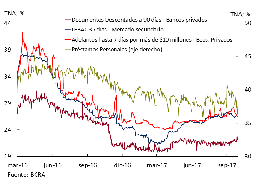
Lending rates continued to show a mixed behavior during the quarter. Considering the average monthly interest rates on loans to the private sector, in the case of financing to companies, the rates on current account advances and signature documents registered increases of 0.6 p.p. and 0.5 p.p., respectively, while the rates on discounted documents remained practically stable between June and September. On the credit side more associated with consumption, the cost of personal loans increased 1.3 p.p. in the same period, while credit card rates registered a slight decrease. Finally, the interest rate on title loans fell 0.3 p.p. in the quarter (see Figure 5.9).
Figure 5.9 | LEBAC rate and bank lending rates
5.3 Exchange rate flexibility and accumulation of international reserves
Since December 2015, the BCRA has implemented a flexible exchange rate regime, an exchange rate scheme that is common in countries that have inflation targeting regimes and that allows the economy to better absorb external shocks (see Section 1 / Exchange rate float and current account volatility). At the same time, the Central Bank intervened in the foreign exchange market by making purchases of foreign currency, with the purpose of reaching a level of international reserves similar to that of other countries in the region that also operate under an inflation targeting scheme and a floating exchange rate regime. This strategy is based on a precautionary demand for foreign currency that can then be used to avoid disruptive volatility of the exchange rate, but which does not have the objective of fixing its level.
During 2016 there were several episodes in which the functioning of this exchange rate scheme could be seen in the face of adverse shocks: the uncertainty associated with Brexit and the result of the elections in the United States, in which the peso depreciated against the dollar. Towards mid-May of this year, the political situation in Brazil had a similar impact on the foreign exchange market, which then lasted until the beginning of August with the expectation of the result of the PASO (primary, open, simultaneous and mandatory elections) in Argentina. The domestic currency depreciated about 15% against the dollar from mid-May to August 11 (the Friday before the elections). As in the episodes of exchange rate volatility in 2016, the rise in the dollar did not have a significant impact on retail inflation in the quarter (see Figure 4.5). This dynamic represents a favorable signal about the credibility of monetary policy, which is key to making exchange rate flexibility an efficient tool for absorbing shocks.
Figure 5.10 | Exchange rate and BCRA interventions in the foreign exchange market
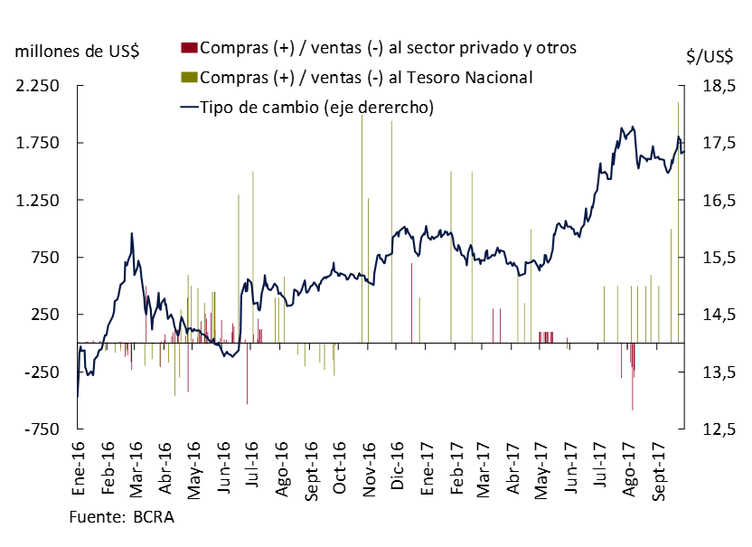
At the same time, in recent months, the usefulness of the strategy of accumulating international reserves to avoid unnecessary uncertainty in the foreign exchange market has become evident. Faced with the sustained rise in the exchange rate in the weeks prior to the PASO, in which market liquidity had been sharply reduced, the Central Bank intervened to moderate exchange rate volatility that was perceived as excessive. Thus, between July 28 and August 11, it sold international reserves on seven occasions for a total amount of US$ 1,837 million (average of US$ 262 million per intervention). The exchange rate against the dollar slowed its upward trend in the days leading up to the primaries, and after the elections it fell 2% until the end of September (see Figure 5.10).
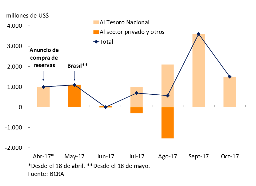
Despite these selling interventions in the foreign exchange market, the purchases of foreign currency from the National Treasury made in the quarter made it possible for international reserves to grow by US$ 2,242 million from the end of June to reach US$ 50,237 million at the end of September. This level represented 8% of GDP, marking a recovery of 4 p.p. of GDP from the bottom of November 2015. Since April 18 of this year, when the Central Bank announced its intention to increase the ratio of international reserves to GDP to 15%, net foreign exchange purchases have been made for an amount close to US$ 7,000 million (see Figure 5.11). 27
Figure 5.11 | Net foreign exchange purchases since the announcement of the international reserves-to-GDP target
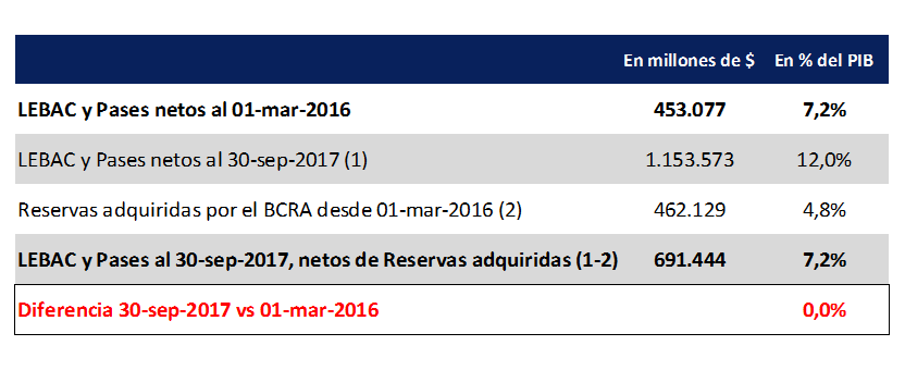
The accumulation of foreign currency has as a counterpart the issuance of bills and net passive passes carried out to sterilize the monetary expansion generated by the purchases of dollars by the Central Bank. These sterilized foreign exchange intervention operations are reflected in an expansion of the monetary authority’s balance sheet. At the same time that non-monetary liabilities (net passes and LEBACs) increase, foreign assets increase. The yield on international reserves, given by the interest rate paid by them and by the evolution of the exchange rate, can offset the financial cost of the liabilities issued to sterilize their acquisition. 28 In this sense, between the beginning of March last year and the end of September of this year, the stock of LEBACs and passes went from 7.2% of GDP to 12% of GDP. However, the purchase of international reserves in the same period reached 4.8% of GDP, so the stock of non-monetary liabilities when the foreign currency acquired is discounted did not change (see Table 5.1).
Table 5.1 | Change in LEBAC stock net of international reserve purchases as of March 2016
5.4 Transfers from the Central Bank to the National Treasury in 2018
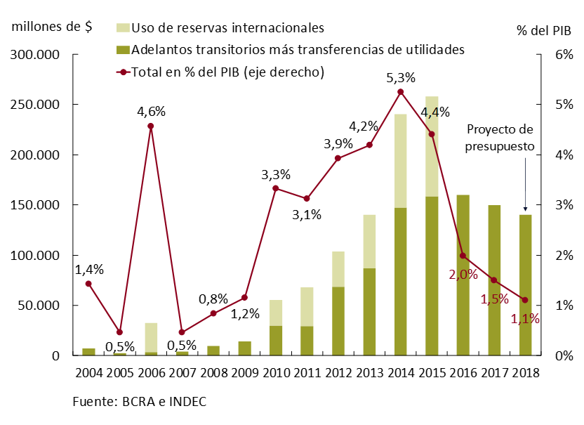
The transfers that the Central Bank will make to the National Treasury in 2018 and that are included in the draft Budget presented in September by the Executive Branch to the National Congress will reach $ 140,000 million. This amount represents a drop compared to what will be transferred during 2017 both in nominal terms ($10,000 million less) and in terms of GDP (it will go from 1.5% of GDP this year to 1.1% of GDP in 2018), which shows the monetary authority’s commitment to its objective of reducing the inflation rate (see Figure 5.12). Likewise, the medium-term fiscal deficit reduction trajectory foreseen by the Ministry of Finance reinforces the downward trend in Central Bank transfers in the coming years and contributes to the objective of reducing inflation.
Figure 5.12 | Transfers to the National Treasury and use of international reserves
This level of transfers to the treasury expected for 2018 will not represent a risk to the evolution of the BCRA’s liabilities and the quasi-fiscal result. Estimates of the demand for money considering the macroeconomic scenario of the National Budget indicate that the amount agreed upon is consistent with the inflation targets for 2018. Moreover, the monetary expansion associated with transfers to the public sector will be lower than the expected increase in the demand for money (by about $20,000 million), so it would be possible to reduce the BCRA’s non-monetary liabilities (net passes and LEBAC) as a proportion of the monetary base if there were no other sources of money issuance.
Section 1 / Exchange rate float and current account volatility
Introduction
Floating exchange rate regimes have the virtue of absorbing macroeconomic shocks, facilitating the internal balance of the economy. Typically, the exchange rate appreciates in the face of excess demand, making domestic goods more expensive, and depreciates in periods of demand shortages, making them cheaper.
In order to study the role of floating exchange rate regimes as automatic stabilizers, this section presents a descriptive empirical exercise that shows evidence about the performance in terms of volatility and the level of the current account balance of those economies that in the period 2000-2013 maintained floating exchange rate regimes.
Proposed exercise
There is an extensive literature in which alternative criteria for identifying exchange rate regimes are developed. Some of these criteria focus on what is the regime announced by the political authorities (de jure criteria) while others focus on the behaviors actually observed (de facto criteria).
On this occasion, we will use the methodology of Levy Yeyati and Sturzenegger (2001, 2003, 2005), who propose a classification of the exchange rate regime based on a cluster analysis, to group countries according to the relative volatility of the exchange rate and reserves, constituting a criterion for selecting the de facto regime. 29 Levy Yeyati and Sturzenegger (2016) expand the classification of regimes for the period 1974 – 2013, while extending the sample of countries. Using this extended classification, we proceeded to identify those economies that during the period 2000 – 2013 adopted a floating regime for more than 70% of the period considered. 30 In this way, a sample of 29 economies with de facto floating regimes was obtained, which are listed in Appendix A.
Two characteristics of the exhibition deserve to be highlighted. First, it is heterogeneous in terms of the level of development achieved by economies. Second, the Eurozone is considered as an aggregate economy with floating exchange rates, so that member countries are eliminated from the sample of economies that did not implement floating regimes. 31 The sample of economies that adopted alternative regimes is presented in Appendix B and consists of 97 cases.
Figure 1 presents the relationship between the average current account balance in terms of output and its volatility for each of the economies considered.
Graph 1 | Average and standard deviation of the current account balance (% of GDP) Period 2000-2013
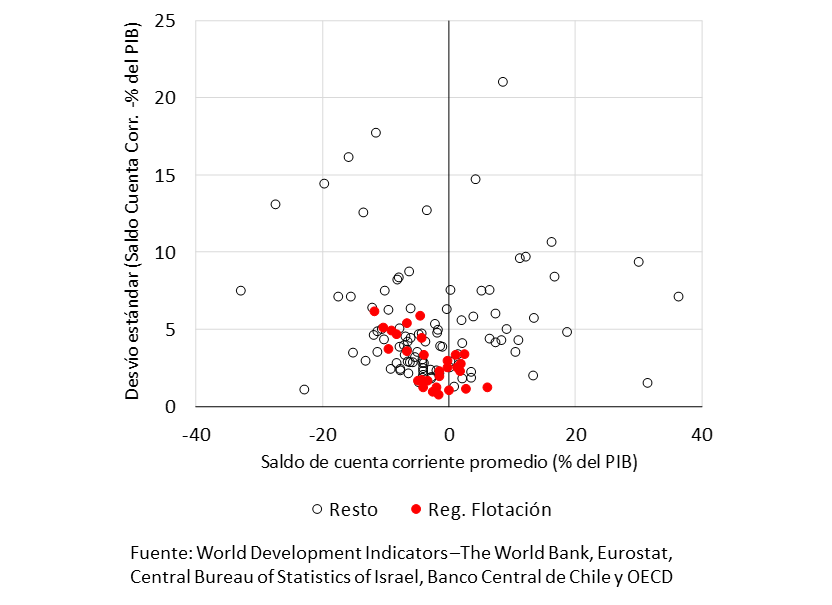
According to the sample analyzed, those economies under floating regimes experienced substantially lower current account volatility. The average standard deviation for economies with floating regimes was 2.83%, while for economies with the remaining regimes it was 5.23%. This lower volatility is associated with the lower prevalence of sudden changes in the current account balance. In turn, economies with floating regimes showed a higher average current account deficit (-2.80%), compared to the -2.06% average of the rest of the cases.
Appendix A
Albania, Armenia, Australia, Canada, Chile, Colombia, Czech Republic, euro area, Hungary, India, Indonesia, Israel, Japan, Kenya, Kyrgyzstan, Madagascar, Mauritius, Mexico, Moldova, Paraguay, Peru, Philippines, Poland, Serbia, Sweden, Tanzania, Thailand, United Kingdom, United States.
Appendix B
Algeria, Antigua and Barbuda, Argentina, Azerbaijan, Bahamas, Bahrain, Bangladesh, Barbados, Belarus, Belize, Benin, Bhutan, Bolivia, Bosnia and Herzegovina, Botswana, Brazil, Brunei, Bulgaria, Burkina Faso, Burundi, Cape Verde, Cambodia, Cameroon, Hong Kong, Macau, China, Comoros, Democratic Republic of the Congo, Congo, Congo, Dominican Republic, Denmark, Djibouti, Dominican Republic, Ecuador, Egypt, El Salvador, United Arab Republic, Gabon, Gambia, Ghana, Guatemala, Guinea, Haiti, Honduras, Iceland, Jamaica, Jordan, Kazakhstan, Republic of Korea, Lebanon, Liberia, Macedonia, Malawi, Malaysia, Mali, Mauritania, Mongolia, Montenegro, Morocco, Mozambique, Namibia, Nepal, New Zealand, Nicaragua, Niger, Nigeria, Norway, Oman, Pakistan, Panama, Qatar, Romania, Russian Federation, Rwanda, Saudi Arabia, Senegal, Sierra Leone, Singapore, South Africa, Sri Lanka, Sudan, Suriname, Swaziland, Switzerland, Syrian Arab Republic, Tajikistan, Togo, Trinidad and Tobago, Tunisia, Turkey, Uganda, Ukraine, Uruguay, Vanuatu, Bolivarian Republic of Venezuela, Vietnam, Zimbabwe.
References
Levy-Yeyati, E. and Sturzenegger. F. (2001) “Exchange rate regimes and economic performance”. IMF Staff Papers 47, 62-98.
Levy-Yeyati, E. and Sturzenegger. F. (2003) “To float or to fix: evidence on the impact of exchange rate regimes on growth”. American Economic Review 93(4), 1173-1193.
Levy-Yeyati, E. and Sturzenegger. F. (2005) “Classifying exchange rate regimes: Deeds vs. words”. European Economic Review, Volume 49, Issue 6, August 2005, Pages 1603-1635.
Levy-Yeyati, E. and Sturzenegger. F. (2016) “Classifying exchange rate regimes: 15 years later”. CID Faculty Working Paper No. 319, June 2016.
Section 2 / An association between cash intensity and construction activity
The evolution of payment systems is the result of innovations that seek to meet the demand for more efficient mechanisms of interaction between economic agents. Globally, a large proportion of transactions are still carried out in cash, and the main causes of this are debated.
One of the BCRA’s objectives is to encourage the massive use of electronic means of payment and facilitate their access to the population as an essential element for financial inclusion. 32 In order to design appropriate policies and measures to facilitate and encourage the use of electronic means of payment, it is important to understand the determinants behind the use of cash in Argentina. Below is the relationship between the intensity of cash use in the economy and construction activity.
Graph 1 | Banknotes and coins/current GDP ratio vs Construction/EMAE ratio (2004-2017)
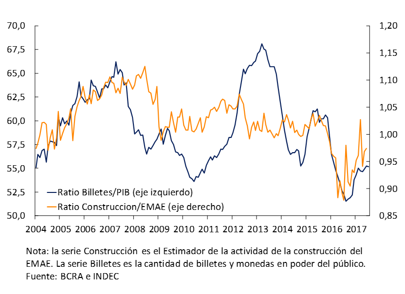
As expected, for transactional reasons there is a positive relationship between the amount of banknotes and coins held by the public in real terms and the size of the economy. However, this relationship is not stable. 33 It was found that the changes in the intensity of the use of banknotes and coins could be explained, in part, by the relative evolution of construction activity with respect to the economy as a whole. 34 This could suggest that different economic activities have different intensity of cash use (see Figure 1).
In order to analyze whether the series are correlated, it is important to know if this does not respond to the existence of a common trend. Therefore, the linear trend of both series is extracted and their cyclical components are analyzed. During the period 2004-2016, the correlation between both variables is positive, with the exception of the period 2011-2015. In the pre-restrictions (Jan-04 to Oct-11) and post-exchange restrictions (Dec-15 to Jul-17) periods, the correlation is positive. In contrast, during the validity of these restrictions, the demand for cash jumped significantly, making the relationship between the two variables negative (Table 1).
To test this relationship, a regression analysis was performed between the cyclical components of both variables. In addition, a dummy variable was incorporated for the period of the clamp that improves the adjustment of the estimate. The results suggest that the coefficient associated with the relative evolution of construction with respect to aggregate activity has a positive sign and is statistically significant to explain the behavior of the intensity of the use of cash.
Table 1 | Banknotes and coins/current GDP vs Construction/EMAE cycle correlations (2004-2017)
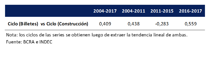
As of the exchange rate normalization (December 2015), the relationship between these variables is significant, with the growth of construction relative to that of economic activity being one of the factors that explains the rise in the intensity of the use of cash during 2016 and 2017.
Section 3 / Public-Private Partnership
Historically, infrastructure works in an economy – such as highways, bridges, airports, and schools – were considered public goods and, as such, were built by governments, financed by taxes, and administered by public bodies. However, since the end of the 80s, several countries began to use Public-Private Partnership (PPP) in some of these developments.
PPP can be defined as an arrangement whereby the government contracts with a private company to build or improve infrastructure works and subsequently maintain and operate them for an extended period of time in exchange for a revenue stream during the term of the contract. Generally speaking, the concessionaire is remunerated with a combination of revenue from the user (a booth on a highway) and/or government transfers (public hospitals). In all cases, at the end of the contract the asset returns to the state orbit35.
Infrastructure projects, such as highways, bridges, tunnels, and ports, are large investments that require a large amount of capital and additionally need to be maintained and operated once built. Therefore, the process by which projects are selected, designed, operated, and maintained is critical. One of the main barriers to growth and development in Latin America has been the insufficient level of infrastructure, which is often reflected in bottlenecks and various inefficiencies, which create obstacles to investment, in turn restricting growth. 36
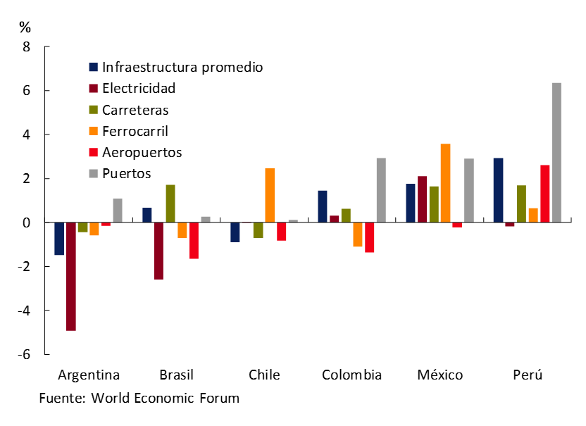
The evolution of infrastructure quality37 in the last decade in the main economies of Latin America37 has shown a heterogeneous behavior by country and by component (see Graph 1).
Graph 1 | Infrastructure quality indicators. Average annual change (2006-2016)
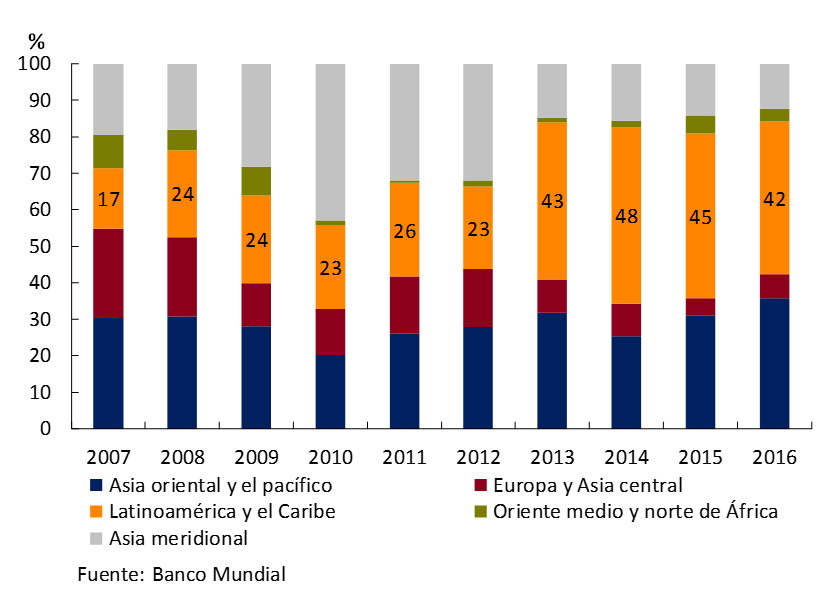
Recognizing that infrastructure investment increases the productivity of all factors of production, improves competitiveness, and increases export capacity, many Latin American countries have turned their attention to infrastructure investment to strengthen their long-term productive capacity through Public-Private Partnershipcontracts 38 (see Figure 2).
Graph 2 | Percentage distribution of PPP projects by region (2007-2016)
In our country, the enactment of the Public-Private Partnership Law39 enabled PPP contracts as a tool for the private sector to finance, build, operate and/or maintain a public good or service, while the State, or the State together with the private sector repay these capital investments and the costs of operation and maintenance in the long term against the provision of a service. PPPs are an alternative to the classic public works contracting systems that aim to develop projects in the fields of Energy and Mining; Transport, Communication and Technology; Water, Sanitation and Housing; and Education, Health and Justice. 40
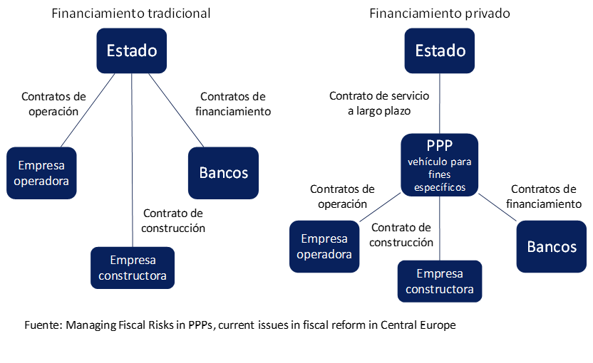
A key difference in comparing the traditional public investment model with that of PPPs lies in the allocation of risk faced by taxpayers represented by the public sector (see Figure 3). In the traditional scheme of infrastructure generation through public works, the funding of projects is based on the cost of government financing, while in PPPs the cost of funding reflects the evaluation of the project’s risk by the private sector and the credit rating of the banks involved. Even in the hypothetical case in which in the latter system (PPPs) the cost could be higher than in the traditional model, taxpayers do not have to face commercial risks, such as those of construction and maintenance of the project, thus modifying the risk/return ratio. Consequently, we could say that, although infrastructure financing through PPPs has the effect of keeping accounts off the balance sheet of public investments, its main benefit is actually its ability to diversify the risks of the parties, take advantage of private sector innovations, and consequently bring greater efficiency to the use of resources.
Graph 3 | Comparison between traditional (Public) and PPP (Private) financing
These operations are not exempt from at least two challenges, according to the literature specialized in the execution and implementation of PPPs in the region. First, the existence of contingent liabilities derived from a poor design of the contract with the private sector may eventually lead the latter to incur losses that force it to carry out a restructuring and it is the public sector that has to assume its debts and liabilities against third parties. 41 Second, if PPP legislation turns out to be inconsistent, situations may arise in which the renegotiation of the contract between the parties undermines PPP efficiency gains and the return on investment. Due to the high occurrence of contractual renegotiation observed in several countries in the region, some countries such as Chile have introduced reforms that limit the renegotiation of contractual renegotiation. 42
Section 4 / Forecasting with Mixed Frequency Models
The Central Bank constantly monitors low and high frequency indicators on the evolution of prices. This section explains the statistical methodology for inferring the evolution of low-frequency data from real-time data. The provincial and “private” price indices turn out to be useful indicators for this purpose, in particular, the IPCBA rest price index prepared by the General Directorate of Statistics and Censuses of the Government of the Autonomous City of Buenos Aires and the index prepared by the company PriceStats in collaboration with State Street Global Markets. 42 The first has a monthly frequency and aims to provide a perspective on the trend of the inflation rate by excluding the direct impact of regulated prices and prices with a marked seasonal behavior; while the second provides a daily indicator of the evolution of the price level based on the compilation of prices from the websites of a multiplicity of businesses in Argentina and their aggregation imitating the methodology of a standard consumer price index.
Graph 1 | Retail Price Indices: Rest IPCBA and State Street PriceStats aggregated monthly
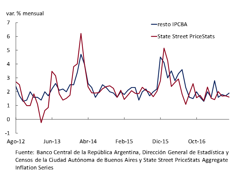
As can be seen in Graph 1, the monthly aggregation of the daily State Street PriceStats index produces a good approximation for the remaining monthly inflation rate of the IPCBA, although slightly more volatile. The question is whether it is possible to combine both indices in a model that allows a short-term prediction of the IPCBA inflation rate. Ghysels et al. (2004)43 propose, in its most simplified version, a simple regression equation that allows us to address this problem,
pi ^C_t = mu + Sigma^{m-1}_{i=0} beta_{i} pi ^{PS}_{t*m-i} + u_{t}
where pi ^C_t represents the core monthly inflation rate, the remainder of the IPCBA (low-frequency), and pi ^{PS}_t, the daily inflation rate of PriceStats (high-frequency), both approximated by logarithmic differences; μ is a constant; m is the number of times the high-frequency variable is observed,44 each beta_i represents the weighting of each day in month45; and u, the residual term.
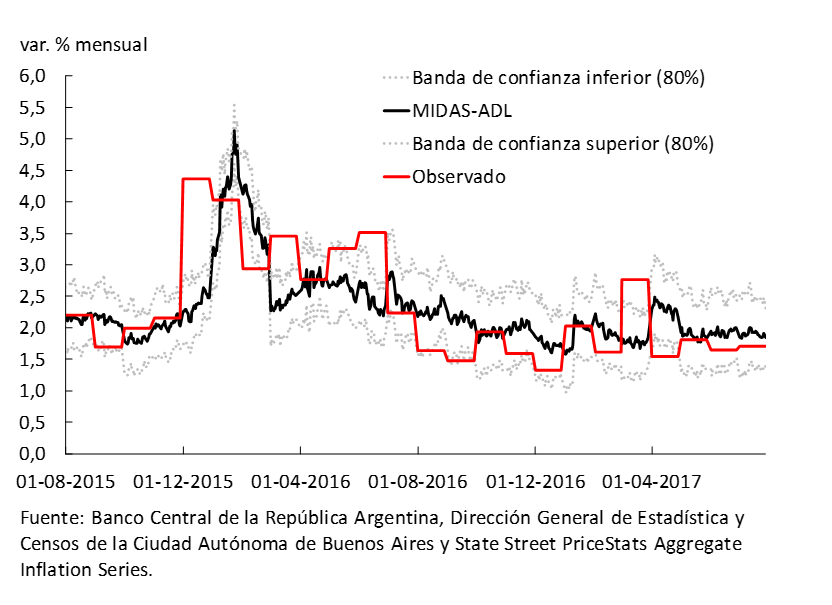
This methodology, known as MIDAS (Mixed Data Sampling Regressions), allows a relatively simple model to combine high- and low-frequency information. Consequently, it is also possible to make intra-period estimates, with a slight modification to the specification of the previous equation, allowing a different forecast to be computed for each day of the month as more information is obtained.
In Graph 2, the performance of this type of model can be contrasted from August 2015 to July 2017 inclusive, carrying out the exercise for Argentina. Two particularities can be highlighted: i) as the inflation rate falls, forecasts become more and more accurate, and ii) as the current month progresses, although there is some volatility, on average the quality of the predictions improves.
Graph 2 | Forecast evolution for the current month
By analyzing point (ii) in more detail, it is interesting to compare the accuracy of this class of models against some other simple model such as an autoregressive model using only the IPCBA low-frequency remainder index or the moving average offered by InflacionVerdadera.com using only the State Street PriceStats high-frequency index.
Graph 3 shows the evolution of the average accuracy of the forecasts considering the period from August 2016 to July 2017 inclusive. The accuracy of forecasts is considered in terms of the square root of the mean square error of forecasts; therefore, a lower value implies a forecast, on average, more accurate.
Graph 3 | Evolution of the average accuracy of IPCBA rest forecasts in the month
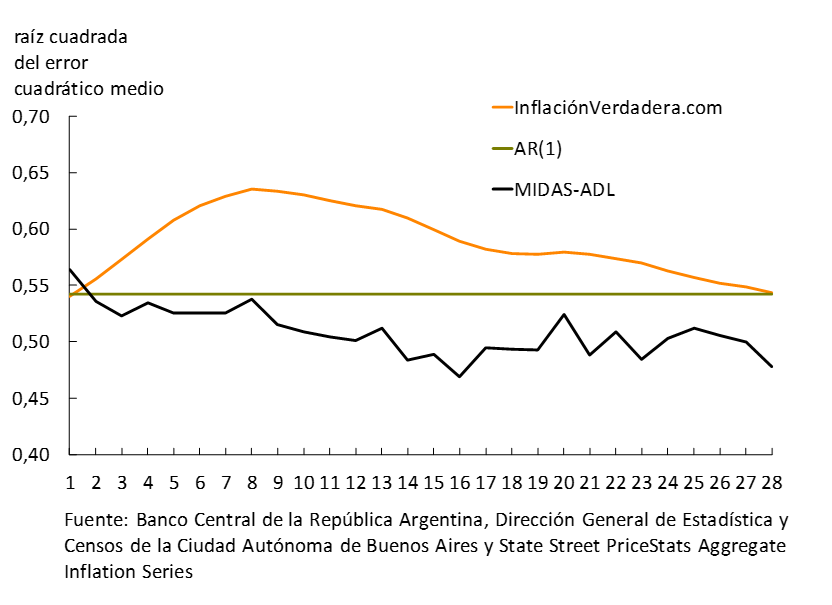
In conclusion, mixed-frequency models perform better than estimators that only consider a single frequency, either the high frequency (State Street PriceStats only), or the low frequency (IPCBA remainder only). Additionally, as observations accumulate within the National Core CPI, recently launched by the new INDEC administration, it will be possible to use these models to predict this index.
Section 5 / The Inflation Targeting Experience in Israel
In the early 1990s, a small number of countries began to adopt the Inflation Targeting (IF) scheme as a monetary policy strategy. Pioneers include New Zealand (1990), Canada (1991), the United Kingdom (1992), Israel (1992), Finland (1993), Australia (1993) and Sweden (1993). Basically, the IM scheme has the following salient features:
• The announcement of an explicit inflation target (or a series of targets over time).
• The commitment of the Central Bank to achieve the goal, which becomes the primary objective of the monetary authority, which in turn must be accountable for the achievement of the proposed objective.
• The adoption of the interest rate as the primary instrument of monetary policy that clearly indicates the bias of the policy and the monetary authority’s stance on inflation. In addition, monetary policy should be carried out based on a forward-looking assessment of inflation dynamics, taking into account inflation forecasts and expectations.
• An institutional transparency strategy that includes monitoring and communicating to the public the monetary authority’s vision.
The theoretical consensus on MI regimes highlights some preconditions that facilitate the success of the regime. 45 Among the preconditions are the operational independence of the monetary authority, the absence of fiscal dominance, the existence of stable and deep domestic financial markets, and that the monetary authority is not committed to objectives on other nominal variables (especially with respect to the nominal exchange rate), among others.
Graph 1 | Israel. Inflation and target
Among the first cases of adoption of IM is the experience of Israel, since unlike the rest of the countries mentioned and contrary to the theoretical consensus, Israel embarked on the path of inflation targeting with an initial level of relatively high and persistent inflation due to a high degree of indexation of the economy. with a fiscal deficit of around 5 points of GDP and with a scheme of relatively narrow exchange rate bands with a decreasing path of devaluation. In fact, the inflation target began to be calculated as a byproduct of the crawling bands of the exchange rate. This is because the rate at which the band limits were adjusted (the minimum rate of currency depreciation) was determined from the differential between the inflation target and the inflation rate of the rest of the world, in order to avoid a constant real appreciation.
As can be seen in Graph I, although disinflation in Israel was a relatively slow process (since it took almost a decade to reduce inflation from levels close to 20% in the early 1990s to single-digit figures only after 1997), it is noteworthy that the adoption of the targeting regime managed to reduce inflation from 20% to 10% in just one year. Likewise, during the first three years of the regime, inflation deviated from the target, both above and below, and the average deviation was 1.03 percentage points.
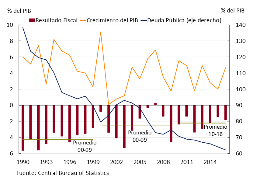
At the same time, on the fiscal front, there was a gradual decrease in the public deficit, which went from an average of 4.2% during the 1990s to 2.2% in the 2010s, indicating that a disinflation program is consistent with fiscal gradualism. Accordingly, the weight of public debt in the economy fell from 120% of GDP in 1992 to just over 60% today.
Graph 2 | Israel. Fiscal deficit and public debt
Among the benefits of adopting the inflation targeting scheme in Israel, in addition to the notable reduction in the rate of price increases and their variability, are having anchored inflation expectations, having broadened the horizon of planning the economy and also having reduced the impact of exchange rate movements on domestic prices.46
Section 6 / Monitoring the mortgage market through internet searches
The use of the Internet as a source of information can be useful both for applied researchers and public officials in monitoring trends in certain markets. There is a high degree of complementarity between traditional statistics and new data sources, although one advantage of the latter is the possibility of having them in near real-time. 47
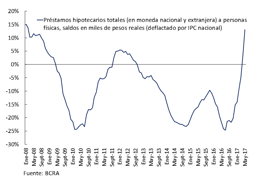
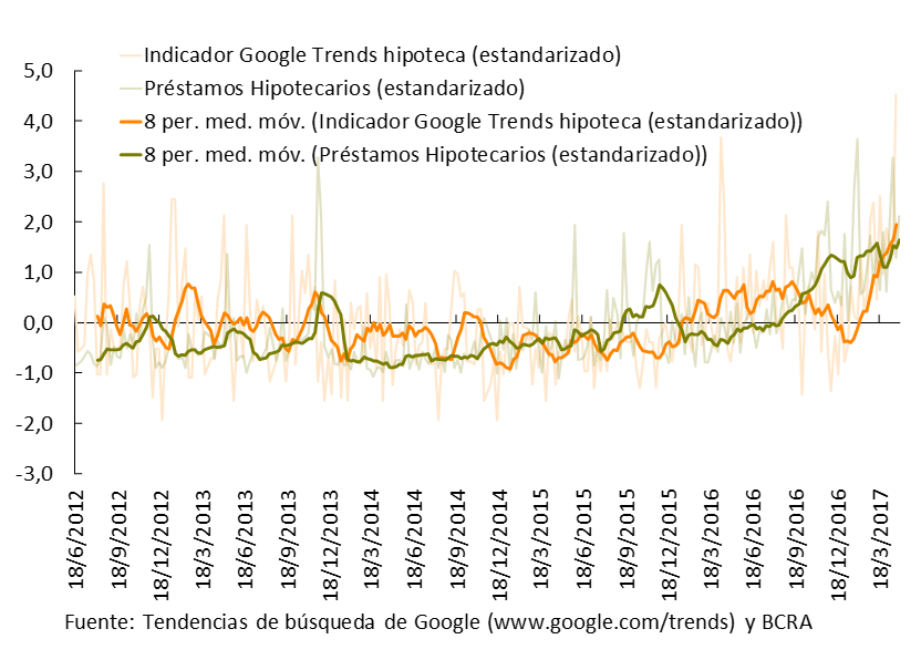
In recent months, the public’s interest in mortgage loans has accompanied their growth rate (see Graph 1), added to a more dynamic real estate market. The objective of the current section48 is to make an application of Google Trends49 to study the demand for apartments and mortgage loans, trying to answer the following question: can we anticipate any aggregate behavior in this market?
Graph 1 | Real stock of mortgage loans. Variation % y.a.
We first briefly describe the data source, then following the spirit of standard exercises in forecasting literature, we study the temporal anticipation of the50 series and whether including the indicator based on Google searches reduces the forecast error. Finally, we present some evidence on loans in Purchasing Value Units (UVA).
Defining the search
Google Trends allows you to monitor social interest in various topics for a defined spatial and temporal scope, through a weekly or monthly time series of the relative search intensity of a specific term. 51 One of its main advantages is that it can condition the research by pre-established categories (one of which is the real estate market) in order to obtain more precise results. With which the first step of the analysis lies in graphing evolution in the intensity of search for apartments for sale compared to apartments for rent. We present these numbers in Graph 2 below.
Graph 2 | Keyword research. Argentina weekly data last 5 years
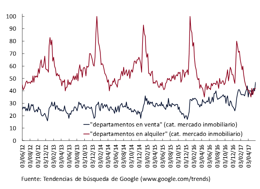
A fact to note is that persistently the search intensity of the term “apartments for rent” is above the search for “apartments for sale”. However, in recent weeks both searches have begun to be more similar and as of mid-March “apartments for sale” surpasses “apartments for rent”.
As a second set of data, we want to see how an indicator built from Google’s results can anticipate the decision to finance the purchase of a home through a mortgage loan. So we work with the values obtained from the search for the term mortgage.
Variable of interest
Next, we must choose a variable of interest to study the explanatory power of search trends. We consider the data on new financing for total mortgage loans (without distinguishing by the type of variable or fixed rate and taking into account both the domestic and foreign currency tranche) to individuals published by the BCRA. Figure 3 presents both series where we filter the noise of working with high-frequency data from moving averages (8 periods).
Graph 3 | Search for mortgages vs New mortgage loans. Last 5 years, weekly data
In more general terms, the link between searches (potential demand) and the performance of acts (deeds) is also interesting. Alternatively, we propose a second exercise taking into account the acts surveyed by the Association of Notaries of the City of Buenos Aires (deeds) and the searches for apartments for sale.
Figure 4 | Searches for apartments for sale vs number of purchase and sale acts. Sample 2004-2017, seasonally adjusted monthly data
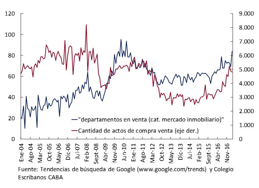
Empirical results
Based on a temporal anticipation test52 , we would be able to affirm that the Google trends variable temporarily anticipates the number of new mortgage loans by approximately 5/6 weeks. When we analyze the search for apartments for sale with the number of deeds, the results also indicate anticipation of the search indicator to the number of deeds in 2 or 3 months.
Following several works in the forecasting literature, we extend an autoregressive model (i.e., one that only looks at the past values of the interest variable), for mortgage loans on the one hand and number of deeds on the other with the indicator elaborated from Google searches (mortgages and apartments for sale).
(1) yt = alpha_0+ alpha_1 y_{t-1} + epsilon_t
(2)yt = alpha_0+ alpha_1 y_{t-1}+ alpha_2 Google Trends_{t-i} + epsilon_t
For the first case, the inclusion of the Google Trends indicator reduces the forecast error (measured by mean square error or RMSE) by 1%. In turn, when we study the effect on the number of writes, the improvement in predictive capacity is 10%. 53
UVA
A phenomenon worth studying is that of loans denominated in Purchasing Value Units (UVA). In recent months, approximately 90% of new mortgage loans are denominated in UVA. This fact can also be seen in the relative interest of this term in Google Trends, as shown in Graph 5.
Graph 5 | Keyword search (UVA Credit) and Mortgage Loans in UVA. Argentina, last 22 months
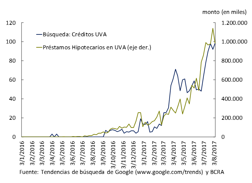
In principle, both series move in a synchronized manner (in fact, they have a correlation coefficient greater than 0.9). Since the series are relatively short, studying the temporal anticipation of one over the other would not yield significant results. However, as more history becomes available, a more detailed analysis will be possible.
Conclusions
The Internet, in particular the searches of individuals in the main engines, opens up a wide range of possibilities to complement the analysis and monitoring of various actors in different markets. Even from a regulatory or normative point of view, it allows us to anticipate certain developments and improve the models currently used in central banks and the public sector.
References
Askitas, N. (2015). “Trend-Spotting in the Housing Market – a significant correlation with the US national S&P/Case Shiller Home Price Index”.
Askitas, N. Zimmermann, K. (2011). “Detecting Mortgage Delinquencies”. IZA Discussion Paper No. 58.
Ayub, P, Raffin, M. (2017). “UVA Mortgage Credits: Is it an instrument that can expand access to housing?”. In Ideas de Peso del BCRA.
Bholat, D. (2015). “Big data and central banks”. BOE Quarterly Bulletin 2015 Q1. Bank of England.
Blanco, Emilio (2014). “Big Data Tools: Can We Leverage Google Trends to Forecast Relevant Macro Variables?” MIMEO, available here.
Coble, D., Pincheira, P. (2017). “Now-Casting Building Permits with Google Trends”. DOI: 10.13140/RG.2.2.36321.10082.
Choi, H., Varian, H. (2011). “Predicting the Present with Google Trends”. Google Technical Report.
Choi, H., Varian, H. (2009). “Predicting initial claims for unemployment insurance using Google Trends”. Google Technical Report.
Dabusti, F. (2017). “UVA loans: the extension of terms becomes more important”. In Ideas de Peso del BCRA.
van Veldhuizen, S., Vogt, B., Voogt, B. (2016). “Internet searches and transactions on the Dutch housing market”. CPB Netherlands Bureau for Economic Policy Analysis Discussion Paper No.325.
References
1The U.S. Federal Reserve (Fed) does not follow a traditional inflation-targeting regime (nor does the European Central Bank, ECB). The Fed has a mandate to promote the goals of “maximum” employment, moderate long-term interest rates, and stable prices. On the latter, at the meeting of the Fed’s Open Market Committee (FOMC) on January 25, 2012, a target of an annual change of 2% was set for the household spending deflator (PCE) in the long term. The ECB seeks to achieve price stability, which it defines as inflation below 2% (but close to that value).
2 See INDEC for Argentina’s main trading partners.
3In all the cases in this chapter, the growth projections of the countries under analysis are taken from the IMF’s World Economic Outlook for October 2017.
4 See Brazil and its Effect on Argentine Activity: A Look at the Commercial Channel, in Ideas de Peso. As indicated therein, this estimate is among the most cautious, with others foreseeing a greater impact.
5 See, for example, Martin Eichenbaum’s presentation at the BCRA’s 2017 Monetary and Banking Conference.
6 For more details, see the corresponding Fed document published on its website.
7 A fall in the terms of trade has an unfavorable impact on Argentina’s trade balance, and an increase has a favorable impact.
8 The trading partner cycle was calculated as a chained arithmetic average with moving weights according to the share of these economies in Argentina’s total exports. In the period 1966-1996, based on the information on total exports of O.J. Ferreres, the following economies were considered: Brazil, the United Kingdom, Chile, China, the Netherlands, Belgium, Germany, France, Italy, Spain, Uruguay, Bolivia, Japan, Mexico, Peru, Paraguay and the United States. For the period 1997-2016, with information from INDEC, the following economies were incorporated: the remaining countries of the euro area, Canada, Colombia, Algeria, Egypt, Indonesia, India, Iran and South Africa. Throughout the entire sample, this group of countries accounted for 66% of total foreign sales.
9 Between December 2011 and September 2017, 3 complete economic cycles were recorded, with different depths and durations. The recessionary phase that began in September 2015 and ended in August 2016 was less profound than the previous two.
10 Composed of machinery, equipment and transport material. .
11 Public consumption also contributed positively (0.2 p.p.), registering an increase of 1.4% s.e. in the second quarter.
12 For more details, see Section 1/ Private consumption, a variable difficult to follow in real time, IPOM July 2017.
13 See section 3.2 of the IPOM activity chapter of July 2017.
14 This is mainly due to the delay in the marketing of maize and soybean products due to climatic factors that affected exports of primary products and MOA.
15 The lending and passive rates set by financial institutions were released. The possible uses of the loanable capacity available in foreign currency were expanded, avoiding currency mismatches in the balance sheets.
16The differences in the rates are contained in the sampling error according to INDEC. The population value of both the employment and unemployment rates are within the range of the confidence intervals of the second quarter of 2016, so it can be inferred that both rates have remained stable between the second quarters of 2016 and 2017.
17 Applying the Hodrick-Prescott filter ((λ: 1600) to the projected GDP series using the REM forecasts for the 10th, 25th, 50th, 75th and 90th percentiles, it is observed that in all cases, analysts implicitly assume a break in the medium-term trend from 2016 onwards.
18 See Highways to Heaven: Infrastructure Determinants and Trends in Latin America and the Caribbean, IMF 2017.
19 This sectoral agreement allows for greater productivity and lower costs, with projected investments of 80,000 million pesos in 2017 and 140,000 million during 2018 related to new drilling and associated infrastructure.
20Law 27,191 declared the generation of electricity from the use of renewable energy sources for the provision of public service to be of national interest, as well as research for technological development and the manufacture of equipment for that purpose. Between the tenders for the Rondas 1 and 1.5 electric power generation capacity, the private companies will invest US$ 4,000 million to install more than 2,400 MW of wind and solar energy.
21 See the BCRA’s Financial Stability Report, First Half of 2017, Section 1.
22 Cerutti, Dagher and Dell’Ariccia, 2017, Housing finance and real-estate booms: a cross-country perspective. IMF staff discussion note, June 2015 and see Warnock, V., and F. Warnock, 2012, “Developing Housing Finance Systems”, Reserve Bank of Australia Annual Conference Volume, Reserve Bank of Australia, Sydney.
23 National coverage price index prepared by INDEC.
24 It represents approximately 70% of the basket.
25 The method used by the Statistics Directorates is that of excluding components, but other statistical measures can also be calculated by applying econometric techniques (for example: principal components and truncated averages; see Section 5 of the IPOM of July 2016).
26 The dynamics of the prices of goods and services in both indicators are similar, both at the monthly level and in the annual cumulative variation.
27 Core component services do not include regulated and seasonal services.
28 In order to assess the nature of monetary policy, it is useful to consider the price indices that measure core inflation. These indicators are a more accurate measure of core inflation. Calculating real rates taking into account core inflation expectations reduces the fluctuations generated by changes in regulated and seasonal prices.
29 This objective is secondary, that is, it is subordinate to that of achieving low and stable inflation, and does not have a defined timetable for compliance. The accumulation of international reserves is a common strategy in many emerging economies that is based on a precautionary demand for foreign currency to avoid disruptive exchange rate volatility (see Section 3 of the IPOM of April 2017: “Strengthening the central bank’s balance sheet: the experience of other emerging economies”).
30 See section 6 of the IPOM of January 2017: “Monetary policy and balance sheet of the BCRA”, of the Monetary Policy Report.
31 For a detailed description of the methodology, see referenced text.
32 As a floating regime, those economies classified as “float” in the first and second rounds of the method were considered – see Levy-Yeyati and Sturzenegger (2016).
33 The exercise proposed in the section was also carried out considering the countries of the Eurozone independently in the sample of the remaining economies, as cases of fixed exchange rate regimes, eliminating the Eurozone from the sample of economies with floating exchange rates. The results obtained do not differ substantially from those presented.
34 See Objectives and plans regarding the development of monetary, exchange, financial and credit policy for the year 2017 (.. /pdfs/institutional/ObjetivosBCRA_2017.pdf.
35 Where we define the intensity of the use of cash as the ratio between the sum of banknotes and coins held by the public and GDP at current prices.
36 Defined as the ratio between the estimator of construction activity and the Monthly Estimator of Economic Activity (EMAE).
37Engel, Fischer and Galetovic. The Economics of Public-Private Partner-ships: A Basic Guide. Cambridge University Press, 2014.
38 Garcia-Escribano, Góes, Karpowicz, 2015, “Filling the Gap: Infrastructure Investment in Brazil,” IMF Working Paper 15/180.
39The World Economic Forum generates the infrastructure quality indicator. This indicator ranges from one (1), very precarious quality, to the upper limit of seven (7) where the infrastructure has good development and efficiency according to international standards.
40 Argentina, Brazil, Chile, Colombia, Mexico and Peru represent 84% of the region’s GDP. WEO, April 2017.
41 PPPs in the region are concentrated in four key types of infrastructure for the region: transport, energy, telecommunications, and water and sewerage supply. Private Participation in Infrastructure (PPI), World Bank, 2016.
42 Law 27.328.
43 According to data from the Public-Private Partnership Unit of the Ministry of Finance, the first 52 projects foresee an investment by the private sector of USD 21,000 million. https://www.minfinanzas.gob.ar/uppp/index.php.
44 See Ehrhardt and Irwin, 2004; Cebotari et al, 2008; Bloomgarden Blumenfeld, 2013.
45See Bitran, Eduardo, Sebastan Nieto-Parra, and Juan Sebastan Robledo, 2013, “Opening the Black Box of Contract Renegotiations: An Analysis of Road Concessions in Chile, Colombia and Peru,” OECD Working Paper No. 317 (Paris: Organisation for Economic Co-operation and Development).
46 The data are partially published on the InflacionVerdadera.com website.
47 Ghysels E., Santa-Clara P., Valkanov R. (2004). “The Midas touch: mixed data sampling regression models”. Working Paper 2004s-20. CIRANO.
48 It is assumed that it is a fixed number; therefore, the observations for the 29th, 30th and 31st of the corresponding months are discarded.
49 To eliminate the resulting proliferation of parameters, it is necessary to apply a polynomial constraint, so that each coefficient is a function of its position within the month and of a fixed number of parameters to be estimated.
50 Eichengreen, Masson, Savastano, and Sharma (1999). “Transition Strategies and Nominal Anchors on the road to Greater Exchange Rate Flexibility”. Essays in international finance, Princeton University. Agénor, Pierre-Richard (2002), “Monetary Policy Under Flexible Exchange Rates: An Introduction to Inflation Targeting,” in Loayza, N. and R. Soto: “Inflation Targeting: Design, Performance and Challenges,” Central Bank of Chile, Santiago, Chile.
51 Leiderman, L. (2000). Monetary Policy Rules and Transmission Mechanisms Under Inflation Targeting in Israel. Research Department, Bank of Israel.
52 It is worth clarifying that working with these new datasets, often of large volume, does not immunize us from the same drawbacks that small samples have: it does not eliminate per se the potential problems of endogeneity or selection bias.
53 For more details see https://ideasdepeso.com/2017/06/26/busquedas-en-internet-googleando-datos/ and https://ideasdepeso.com/2017/09/15/en-busqueda-de-un-credito-hipotecario/.
54 For more details, visit https://trends.google.com.ar/trends/ or consult Choi, H. and H. Varian (2011). “Predicting the Present with Google Trends”. Google Technical Report.
55 Through a Granger Causality Test. Specifically, what the test evaluates is whether one time series (with its leads and lags) temporarily anticipates another.
56 First, the number of searches for a keyword or phrase is normalized by dividing it by the total number of searches on Google (controlling for geographic region, date, and selected category). Subsequently, it is re-scaled in such a way that the quotient takes a value equal to 100 for the maximum popularity within the analyzed sample.
57 For reasons of space, the results of the causality test are not presented here, but they are available to anyone who requests them.
58 The out-of-sample forecast for the period 2015m1-2017m7 is evaluated from a sample of rolling windows for the different models, where the i arises from the results of the temporal anticipation. Again, the results are available to anyone who requests them.
Glossary of abbreviations and acronyms
€: Euro
Acum.: Cumulative
AFCP: Portland Cement Manufacturers Association
AFIP: Federal Administration of Public Revenues
AUH: Universal Child Allowance for Social Protection
BADLAR: Buenos Aires Deposits of Large Amount Rate (interest rate paid for fixed-term deposits of more than one million pesos in the 30 to 35-day bracket by the average of banking entities)
BCB: Central Bank of Brazil
BCBA: Buenos Aires Stock Exchange
ECB: European Central Bank
BCRA: Central Bank of the Argentine Republic
BONAR: Argentine Nation Bond
CABA: Autonomous City of Buenos Aires
CEMBI+: Corporate Emerging Market Bond Index Plus
CEMBI+AR: Corporate Emerging Market Bond Index Plus Argentina
ECLAC: Economic Commission for Latin America and the Caribbean
CER: Reference Stabilization Coefficient
FIGURE: Research and Training Center of the Argentine Republic – Central de Trabajadores de la Argentina (CTA)
COICOP: Classification of Individual Consumption According to Purpose
CNV: National Securities Commission
Contrib.: Contribution
S Fuels Energy
DJVE: Affidavits of Foreign Sales
e: Dear
EDP: Durable Production Equipment
EIL: Survey of Labor Indicators
EMAE: Monthly Estimator of Economic Activity
EMBI+: Emerging Markets Bond Index Plus
EMBI+AR: Emerging Markets Bond Index Plus Argentina
EMBIG: Emerging Market Bond Index Global
ENGHo: National Survey of Household Expenditure and Income
EPH: Permanent Household Survey
excl.: Excluding
Fed: Federal Reserve of the United States
FIEL: Latin American Economic Research Foundation
IMF: International Monetary Fund
IMF WEO: World Economic Outlook
FOB: Free on Board (purchase and sale operations carried out by boat)
FOMC: Federal Open Market Committee
GBA: Greater Buenos Aires
A.I.: Year-on-year
IAMC: Argentine Institute of Capital Markets
IBIF: Gross Domestic Fixed Investment
ICC: Consumer Confidence Index prepared by the Torcuato Di Tella University
ICC-INDEC: Construction Cost Index
IGA-OJF: Orlando J. Ferreres General Activity Index
ILA: Activity Leader Index
ILCO: BCRA’s Leading Indicator of Private Consumption
INDEC: National Institute of Statistics and Censuses
INML: Liniers Market Steer Index
CPI: Consumer Price Index of national coverage released by INDEC
IPCBA: Consumer Price Index of the City of Buenos Aires
CPI Cordoba: Consumer Price Index of the Province of Cordoba
CPI GBA: Consumer Price Index of Greater Buenos Aires
CPI-NP: Weighted National Indicator
San Luis CPI: Consumer Price Index for the Province of San Luis
IPIB: Basic Domestic Price Index
IPIM: Internal Wholesale Price Index
MPPI: Commodity Price Index
IPOM: Monetary Policy Report
ITCNM: Multilateral Nominal Exchange Rate Index
ITCRM: Multilateral Real Exchange Rate Index
VAT: Value Added Tax
kg: Kg
LAC: Latin American Consensus Forecasts
LEBAC: Central Bank Bills (Argentina)
LFPIF: Financing Line for Production and Financial Inclusion
M2: Banknotes and coins + quasi-currencies in circulation + current accounts in $ and savings accounts in $
Mens.: monthly
MERVAL: Buenos Aires Stock Exchange
mill.: Million
Min.: Ministry
IPM: Input-output matrix
MOA: Manufactures of Agricultural Origin
MOI: Manufactures of Industrial Origin
MRO: Main refinancing operations
MSCI: Morgan Stanley Capital International Index
MULC: Single and Free Exchange Market
NEA: Northeast Argentina
NG: General level
NOA: Northwest Argentina
OECD: Organisation for Economic Co-operation and Development
OPEC: Petroleum Exporting Countries
bp: Basic points
p.p.: Percentage points
p: Projected
PAMI: Social Work for Retirees and Pensioners
PCE: Personal consumption expenditures
PCP-BCRA: Contemporary BCRA GDP Prediction
EAP: Economically Active Population
GDP: Gross Domestic Product
PMI: Purchasing Managers’ Index
PP: Primary Products
Prom. Moving Average: Moving Average
Avg.: Average
R$: Real
REM: BCRA Market Expectations Survey
REPO: Repurchase Agreement (Operación de Recompra)
ROE: Records of Export Operations
REPO Round: Average interest rate of 1-business day transactions between financial institutions in the guaranteed market
S.A: Sociedad Anónima
s.e.: Series without seasonality
SSPM: Private Consumption Indicator prepared by the Ministry of Finance
TFF: Federal Funds Rate
tonnes: tonnes
TN: National Treasury
APR: Annual Nominal Rate
Trim.: Quarterly / Quarter
ICU: Utilization of installed capacity
US$: US Dollars
UTDT: Universidad Torcuato Di Tella
UVA: Unit of Purchasing Value
Var.: Variation
Vol.: Volume
YPF SA: Yacimientos Petrolíferos Fiscales Sociedad Anónima
Share on


