Summary
As indicated in its Organic Charter, the Central Bank of the Argentine Republic “aims to promote, to the extent of its powers and within the framework of the policies established by the National Government, monetary stability, financial stability, employment and economic development with social equity”.
Without prejudice to the use of other more specific instruments for the fulfillment of the other mandates – such as financial regulation and supervision, exchange rate regulation, and innovation in savings, credit and means of payment instruments – the main contribution that monetary policy can make for the monetary authority to fulfill all its mandates is to focus on price stability.
With low and stable inflation, financial institutions can better estimate their risks, which ensures greater financial stability. With low and stable inflation, producers and employers have more predictability to invent, undertake, produce and hire, which promotes investment and employment. With low and stable inflation, families with lower purchasing power can preserve the value of their income and savings, which makes economic development with social equity possible.
The contribution of low and stable inflation to these objectives is never more evident than when it does not exist: the flight of the local currency can destabilize the financial system and lead to crises, the destruction of the price system complicates productivity and the generation of genuine employment, the inflationary tax hits the most vulnerable families and leads to redistributions of wealth in favor of the wealthiest. Low and stable inflation prevents all this.
In line with this vision, the BCRA assumes as its primary objective to reduce inflation. As part of this effort, the institution publishes its Monetary Policy Report on a quarterly basis. Its main objectives are to communicate to society how the Central Bank perceives recent inflationary dynamics and how it anticipates the evolution of prices, and to explain in a transparent manner the reasons for its monetary policy decisions.
1. Monetary policy: assessment and outlook
On October 1, 2018, the new monetary policy regime came into force, in which the Central Bank of the Argentine Republic (BCRA) committed not to increase the monetary base until June 2019, with the exception of December 2018 and June 2019 when there is an increase in the demand for money. This regime, which was introduced at a time of high nominal instability, establishes a concrete and powerful commitment, immediately observable and verifiable by the public.
The BCRA implements the new regime by holding daily auctions of Liquidity Bills (LELIQ) with banks. The BCRA exceeded the monetary base target in all the months since the launch of the new regime. These over-compliances were 19 billion pesos in October, 15 billion pesos in November and 14 billion pesos in December.
The average interest rate on LELIQs stood at 73.5% annually at the beginning of October, and fell to 56.9%, the latest available data on January 22. The largest decrease in inflation occurred during the month of November, due to the effect of the reduction in nominal volatility, inflation expectations and the general price level of September and October. The decline in the interest rate slowed down as of December, given the recovery evidenced by the circulating currency held by the public in that month, which grew even above the usual seasonal factor of that period and in contrast to the trend that had been verified since the beginning of 2018. Fixed-term deposits, on the other hand, grew strongly in the quarter, favored both by the level of the reference rate and by the incentive to transmit it to the system’s passive rates generated by the minimum cash regulations in force since October 1.
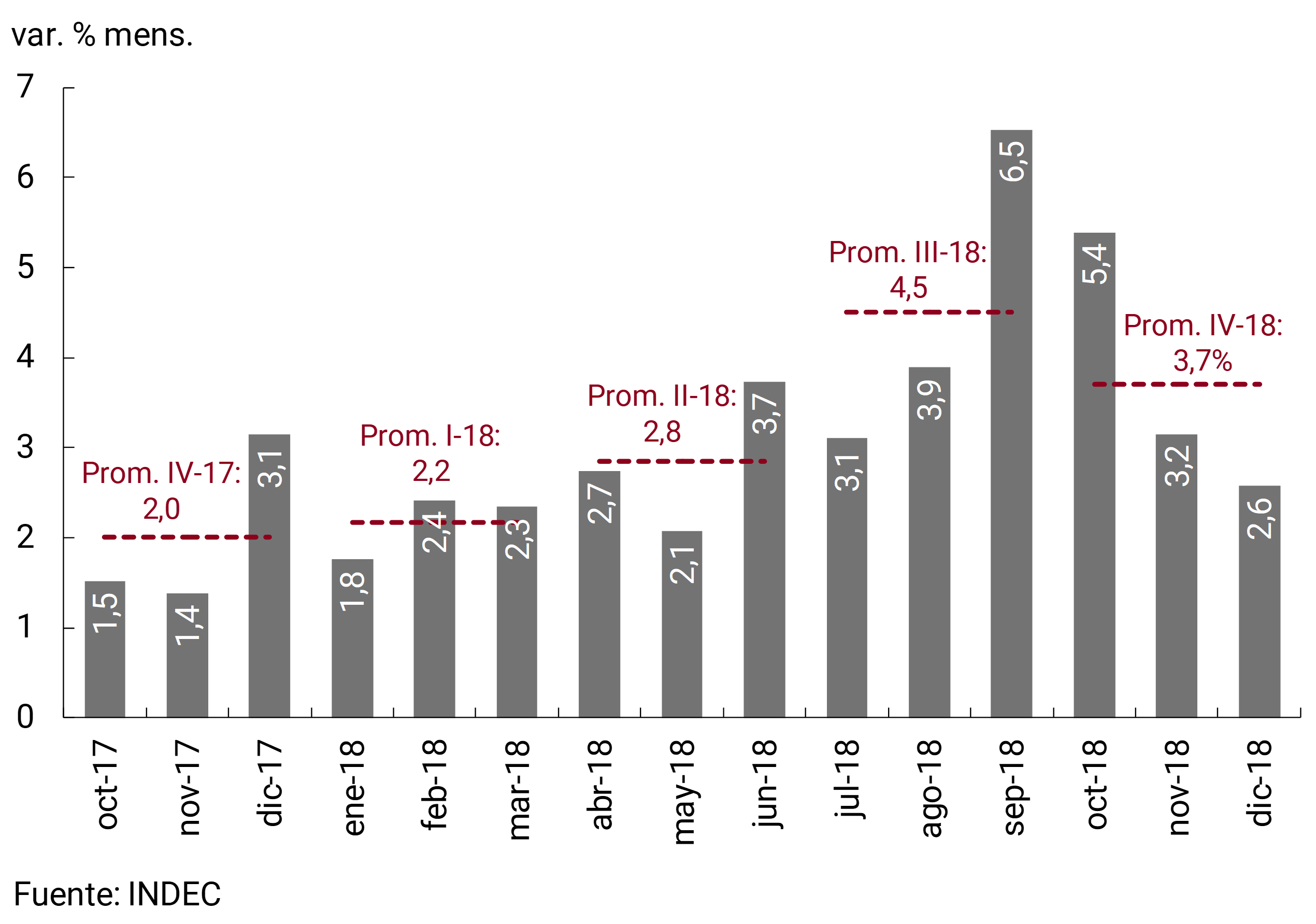
Monthly inflation records fell from 6.5% in September and 5.4% in October, to 3.2% in November and 2.6% in December. The contractionary bias of monetary policy, reinforced by the new regime in force, has allowed nominal control of the economy to begin to be retaken. In any case, inflation is still at high levels. It is known that monetary policy operates with lags. Analysts expect the monthly inflation rate to remain high in the coming months and the regulated price adjustments announced for the near future impose additional conditioning in that regard.
In the current monetary policy scheme, the monetary base objective is complemented by the definition of foreign exchange intervention and non-intervention zones for the exchange rate. The foreign exchange non-intervention zone was defined on October 1, 2018 for an exchange rate of 34 pesos per dollar at the lower limit and 44 pesos per dollar at the upper limit. These limits were adjusted daily at a rate of 3% per month in the last quarter of 2018, and are being adjusted at a rate of 2% per month in the first quarter of 2019. Above the non-intervention zone, the BCRA can make foreign currency sales of up to 150 million dollars per day, generating an additional monetary contraction at times of greater weakness of the peso. On the other hand, the BCRA can make purchases of foreign currency when the peso appreciates and is below the non-intervention zone. Within this zone, the exchange rate fluctuates freely. This system adequately combines the benefits of exchange rate flexibility to face real shocks with the possibility of limiting excessive and disruptive fluctuations that may appear in a still shallow exchange market like ours.
The exchange rate has remained within the non-intervention zone during the last quarter of 2018, although approaching the lower bound. During the month of January, in which the effects of the current monetary policy and a more favorable international context for emerging markets are combined, the exchange rate was below the non-intervention zone and the BCRA began to buy foreign currency, accumulating a total of 290 million dollars until the publication of this report. As it had announced at the beginning of the month, the BCRA limited itself to buying no more than 50 million dollars per day during January, considering it the appropriate limit for the monetary dynamics expected for that month. The monetary expansion associated with the purchases implies a partial increase in the monetary base target in January (5,360 million pesos), as it is in force on only some days of the month from which operations are carried out. This increase in the target becomes full in February (10,819 million pesos).
During the last quarter of 2018, with a more competitive exchange rate parity and a lower level of activity, the Argentine economy made a significant adjustment to its current account deficit. The BCRA estimates that the annualized deficit for the quarter (without seasonality) would be at levels close to 1.2% of GDP, when it came from levels above 6%. This correction of the external imbalance is a fundamental ingredient from which a process of growth can begin on a more solid basis.
The BCRA’s interest-bearing liabilities, mainly composed of LELIQ since the dismantling of LEBAC, remained stable in nominal terms in the quarter. The interest paid on these liabilities was offset by the reduction in its stock made in December to meet the seasonal increase in the monetary base contemplated in the monetary scheme. In terms of GDP or international reserves, the BCRA’s remunerated liabilities fell significantly.
The BCRA’s view is that the monetary plan in force since October 1 has made it possible to begin to reduce the nominal volatility that had occurred in previous months. The monthly inflation rate has fallen from the levels of September and October, but is still at a high level. The BCRA will continue to act with prudence and perseverance to ensure that this evolution is consolidated.
2. International context
The conditions of access to international financial markets for emerging economies, which had begun to deteriorate rapidly in 2018, had a slight improvement in the margin. Thus, the depreciation of emerging market currencies stopped and a net inflow of capital to these markets was recorded. This is partly explained by the slowdown in the tightening of monetary conditions in the United States, which translates into more favorable prospects for 2019 for emerging economies. However, economies with pronounced external imbalances and/or high levels of indebtedness continued to face adverse financial conditions.
During the last quarter of 2018, a positive performance of global economic activity continued to be observed, including in Argentina’s largest trading partners. In the main developed markets (the United States, the euro area (Germany in particular), and in China among the emerging markets, there was a slowdown in their expansion rate in the latter part of 2018. However, the estimated growth of Argentina’s most important trading partners, mainly boosted by the higher level of growth expected for Brazil, pari passu with the projected levels of the real exchange rate, allow us to expect an improvement in the performance of the Argentine external sector, with positive impacts on the level of local activity for 2019.
Therefore, a mixed international scenario is observed for Argentina. On the one hand, the external financial scenario continues to be adverse for some emerging economies, while the commercial channel is expected to give some boost to the level of local activity in 2019. Even more contractionary international financial conditions, together with a deepening of protectionist measures, continue to be the main risks of the international scenario facing the local economy, although as analyzed in the chapter it is less likely than in recent months that these risks will materialize. A new risk factor that is emerging on the international stage is a possible slowdown in the level of global activity.
2.1 Improving the level of activity of our trading partners, mainly Brazil
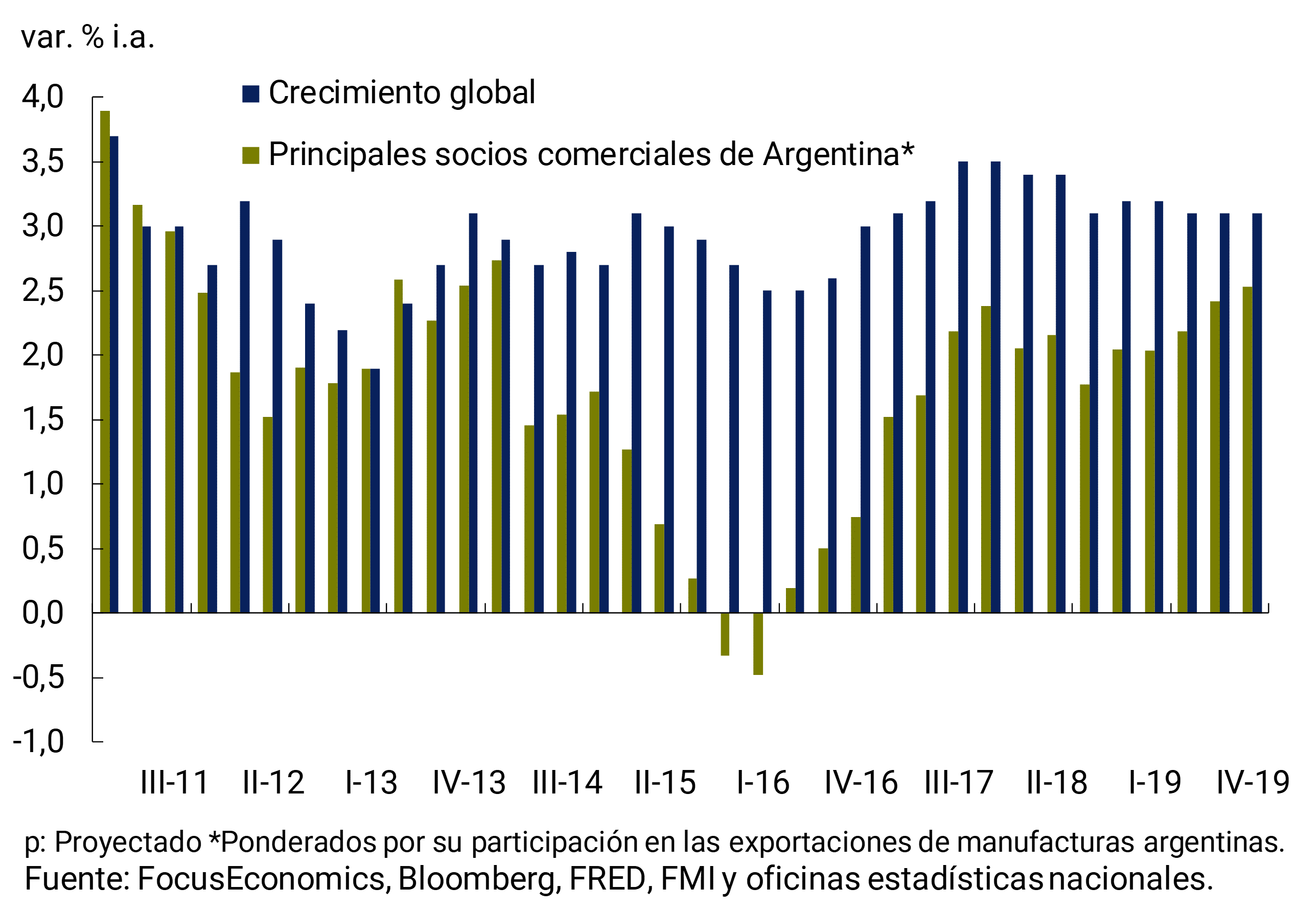
The most recent projections show an expected growth rate of the global economy of 3.5% for 2019, being the same less synchronous than in previous years. Argentina’s main trading partners are expected to increase their growth slightly (especially due to Brazil), with 2019 expected to be the highest value in the last six years (see Figure 2.1). This would have a positive impact on the level of local activity. However, some data would be beginning to show increasing chances of a recession in the world’s largest economy (the United States), which would clearly affect the level of global activity. Indeed, the rate differential between the 10-year bond and the 3-month bond of the United States indicates that the probability of having a recession in December 2019 would be 21.4%, double what was observed a year ago (see Section 1).
Figure 2.1 | Growth of Argentina’s trading partners
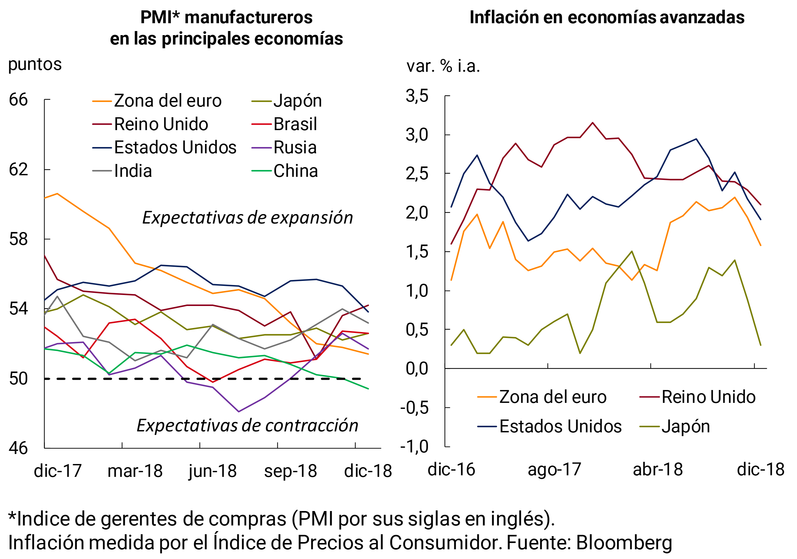
On the other hand, we are also beginning to observe a lower dynamism in the leading indicators of the industry of the main economies. In all cases, the PMI indices, although they are in the expansion zone (except in China, which is already in the contraction zone), as of December 2018 they are at values markedly below those of a year ago with a tendency to go to the contraction zone (except in Brazil). In contrast to the previous quarter, inflation rates in the surveyed economies are below or at target (United Kingdom, see Figure 2.2). This would give some leeway to its monetary authorities, which is in line with the slight improvement observed in global financial conditions.
Figure 2.2 | Leading indicators of manufacturing activity and inflation
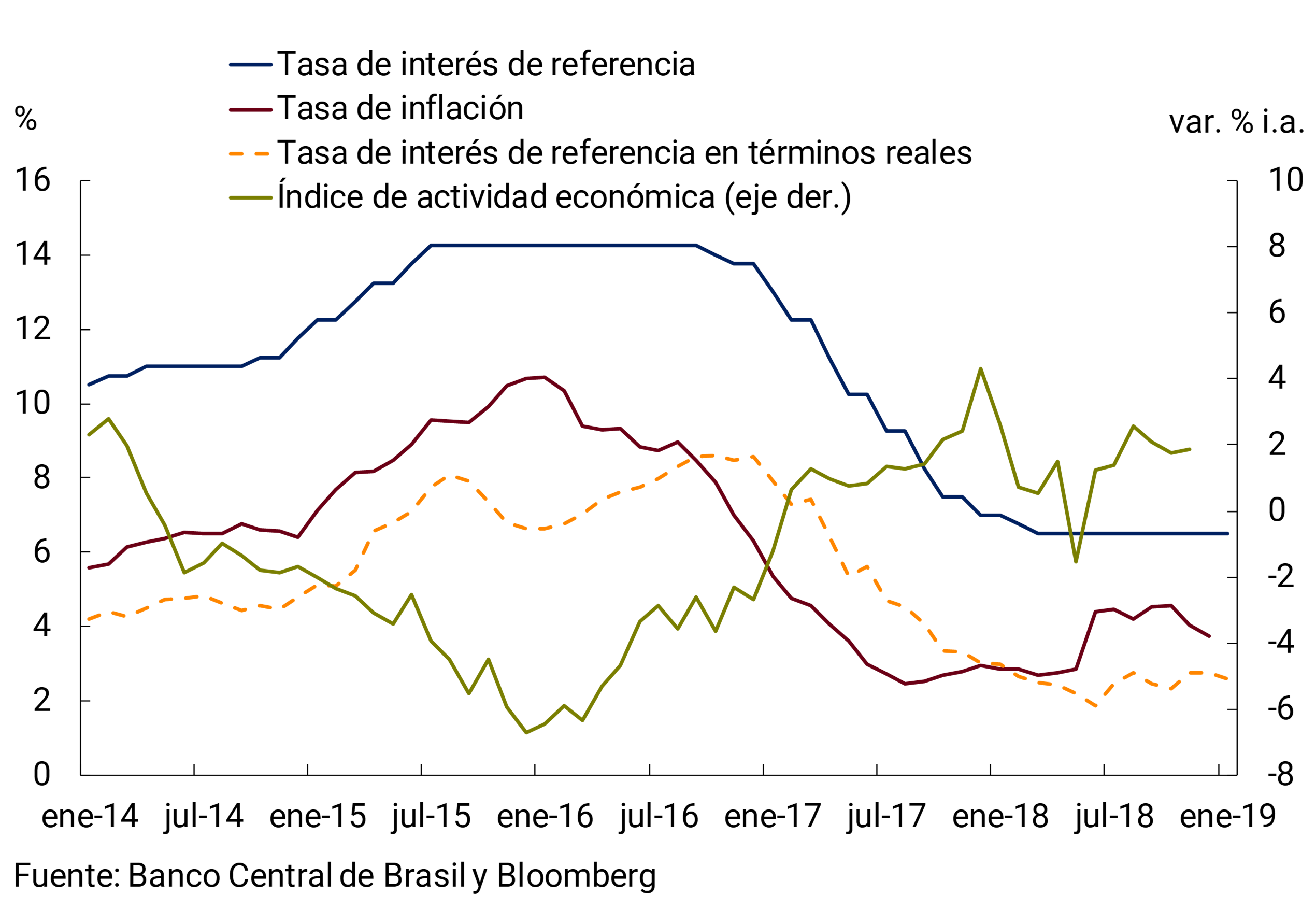
Brazil’s activity indicators recovered after the May low (linked to union strikes). GDP in the third quarter grew 0.8% without seasonality (compared to the previous quarter), being the highest growth rate in the last six quarters. In the same sense, the monthly activity data measured by the IBC-Br estimator of the Central Bank of Brazil (BCB) show year-on-year growth rates of 1.9% in November (without seasonality). The latest estimates for 2018 from the BCB’s Focus survey foresee growth for 2018 of 1.3%, while for this year a GDP increase of 2.5% is projected, which would be the highest growth since 2013. The realization of these forecasts would imply a favorable impact on bilateral trade, and therefore on Argentina’s GDP this year (see Chapter 3).
The BCB recently made no changes to the monetary policy interest rate, which stands at 6.5% (see Figure 2.3). For its part, year-on-year inflation in December was 3.8%, below the center of the target (4.5% ± 1.5). Thus, after the increase in year-on-year inflation in June, linked to union force measures, the inflation rate remained in the last seven months at levels close to the center of the target (4.3% on average). According to the projections of the analysts revealed by Focus, the inflation rate would end 2019 without major changes at 4%, while the BCB would increase the monetary policy rate by 0.5 p.p. (in October 2018 Focus analysts predicted an increase of 1.5 p.p.). For its part, the volatility of the exchange rate, which had increased on the eve of the electoral process, was reduced after the end of the electoral process. The real had a slight tendency to depreciate after the second round of the elections (end of October), which had been reversed in mid-January 2019.
Figure 2.3 | Brazil. Macroeconomic indicators
In the euro area, the slowdown in economic activity that began in early 2018 continued. After having grown at a rate of 0.7% (compared to the previous quarter and without seasonality) in all quarters of 2017, GDP grew 0.4% in the first and second quarters of 2018, and 0.2% in the third (see Figure 2.4). In part, the slowdown in the last quarter was linked, according to the European Central Bank (ECB), to lower automotive production due to the implementation of the Worldwide Harmonised Light Vehicle Test Procedure (WLTP)1. Mainly for this reason, German GDP contracted by 0.2% in the third quarter2. A slowdown in domestic demand was another factor influencing the euro area’s lower growth. However, according to the latest projections, the level of activity in the euro area would improve slightly in 2019 and 2020, around 0.5% QoQ (1.7% YoY) for 2019, and 0.4% QoQ (1.7% YoY) for 2020. Despite the slowdown in the growth rate, labor market data show the lowest unemployment rate (7.9%) since October 2008.
Figure 2.4 | Euro area. GDP growth

As expected, throughout the quarter the ECB did not modify its monetary policy interest rate, which applies to Main Refinancing Operations (MRO), and which remains at an all-time low of 0%, nor did the rate corridor. In addition, no change in policy interest rates (MROs) is expected for most of 2019, despite the fact that the ECB ended its quantitative easing programme at the end of 2018 3.
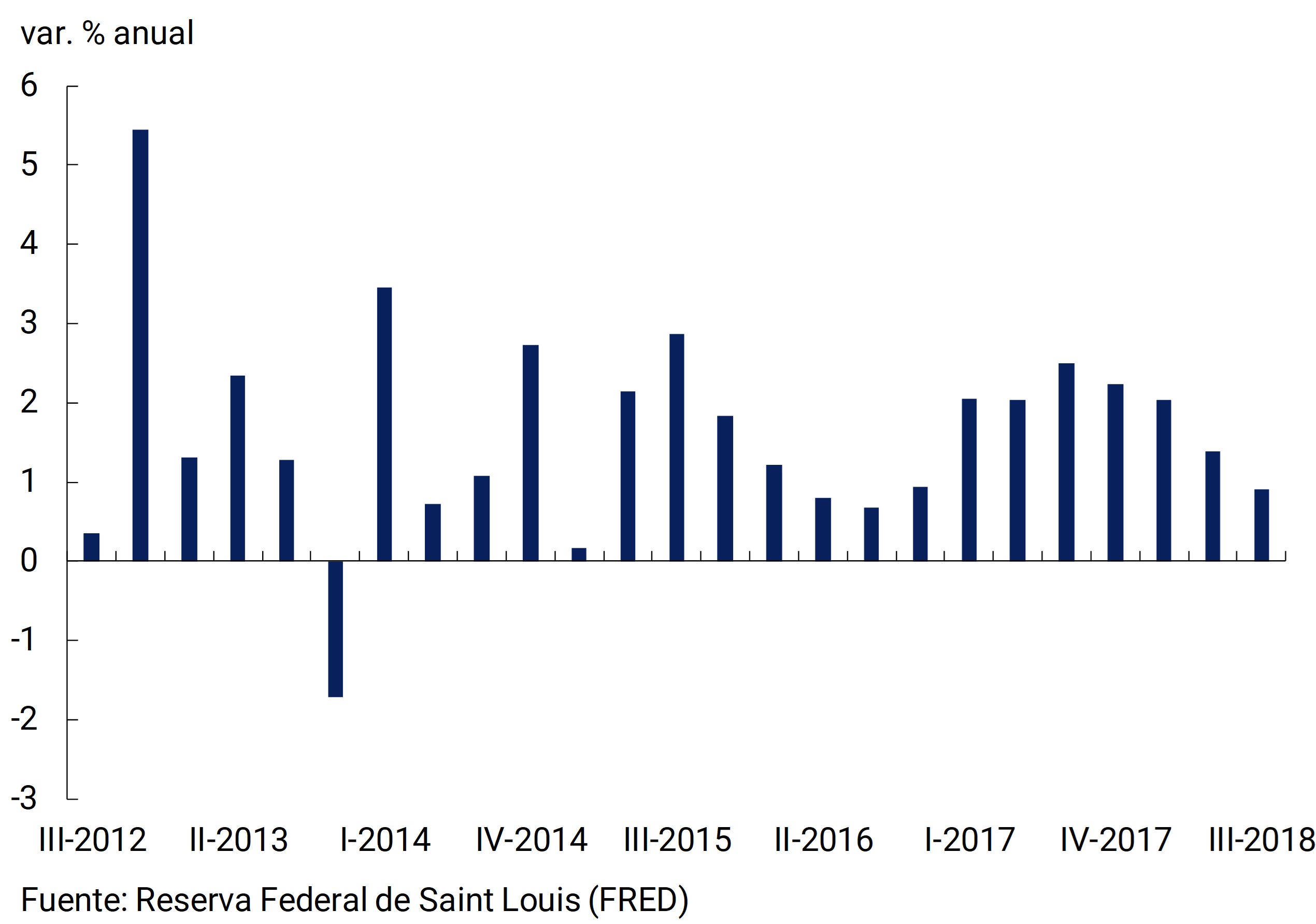
Figure 2.5 | United States. Disaggregated change in GDP

In the United States, the growth rate in the third quarter was 3.4% (seasonally and annualized, see Figure 2.5). This lower rate compared to the previous quarter is explained, among other factors, by net exports, which went from a contribution to growth of 1.2 to -2 p.p. Some leading indicators such as the Atlanta Federal Reserve’s GDPNow are showing that the growth rate of the US economy in the fourth quarter would continue to slow towards values around 2.8%. Unemployment stood at 3.9% in December (the lowest value since January since 1970). On the other hand, unit labor costs, which from the first quarter of 2017 to the second quarter of 2018 had been growing at an average of 2% year-on-year, reduced their growth rate to 0.9% in the third quarter (see Figure 2.6).
Figure 2.6 | USA. Non-farm unit labour cost
The Fed’s Monetary Policy Committee (FOMC) increased, again and as expected, at its December meeting the benchmark interest rate4 to the range of 2.25-2.5% (0.25 p.p.). Thus, by the end of 2018 the benchmark interest rate in real terms would have been positive again for the first time in more than a decade (since September 2008). The FOMC stopped calling its monetary policy expansionary since the September press release. From the latest projections released by the FOMC, it is expected to increase its benchmark interest rate twice in 2019 to the range of 2.75-3% (0.25 p.p. each time). However, in early January, signals emerged both in the futures markets and from some FOMC members, that the Fed’s benchmark interest rate could be increased only once in 2019 or even remain unchanged, and also, if necessary, the Fed’s asset tightening could be paused. All this helped the improvement in international financial markets that has been observed since the beginning of January, as discussed in the next section.
In addition, in the December 2018 projections of the FOMC, there were no significant changes with respect to what was projected in September, either in activity (growth and unemployment), or in inflation. Thus, GDP is expected to grow 2.3% (-0.2 p.p.) in 2019, and 2% in 2020, unemployment to be 3.5% in 2019, and 3.6% in 2020, and inflation to be 1.9% (-0.1 p.p.) in 2019 and 2.1% in 2020. However, some multilateral organizations expect lower GDP growth than the FOMC expects, especially for 2020 (1.8%). In part, this may be due to the fact that the positive effects on growth of expansionary fiscal policy and trade restrictions on China would be extinguished in 2020.
Figure 2.7 | China. GDP growth

Growth in China, the main destination for Argentina’s primary commodity exports, continued to slow throughout 2018, partly due to the impact of trade tariffs imposed on its exports to the United States5. Specifically, GDP in 2018 grew 6.6%, the lowest value since 1990. This lower growth was mainly due to the poor performance of the external sector, partially offset by domestic absorption. In this context, at the beginning of January the central bank of China again reduced reserve requirements on the financial system. Similarly, in mid-January the Chinese authorities announced a reduction in the VAT rate (and other taxes) on some branches of industry, along with an increase in infrastructure spending. The most recent projections show that for both 2019 and 2020, GDP growth of 6.2% is expected (unchanged from previous projections).
2.2 The external financial scenario had a slight improvement in the margin, the doubt is whether it will only be temporary
Although global liquidity conditions remain accommodated in historical terms, they had begun to tighten rapidly over the past year. However, some indicators in the financial markets indicate that in recent weeks this process has been slowing down. However, there are still considerable risk factors for the coming months, although less likely than in the previous IPOM due to what has been analysed so far. Among them: 1) that inflationary pressures in the United States lead to a further tightening of monetary conditions in that country, which are reflected in an increase in the yield rate of its long-term treasury bonds; 2) that the dollar resumes the tendency to appreciate for much of 2018, driven by the decoupling in monetary policy cycles, having as a counterpart a renewed boost to the outflow of capital from emerging markets; 3) that the current trade tensions produce a further slowdown in the Chinese economy that drives a depreciation process of the yuan, and that this spreads to the rest of the emerging markets; 4) Finally, the level of public and private debt in some developed countries, together with the current level of asset prices (both financial and real) in some markets, has the potential to be a disruptive factor for global financial markets, if it leads to a deterioration in investor confidence.
During the fourth quarter of 2018, emerging countries faced sovereign and corporate risk premiums higher than in recent years, reflecting the rise in the cost of external financing in capital markets. The amount of gross debt issuances (sovereign and corporate) of emerging countries in international markets showed a contraction of 33% year-on-year in the fourth quarter, basically due to company placements (with a decrease of 45% year-on-year), as sovereign placements were more stable (with an increase of 2%).
Figure 2.8 | Sovereign and corporate debt risk indicators
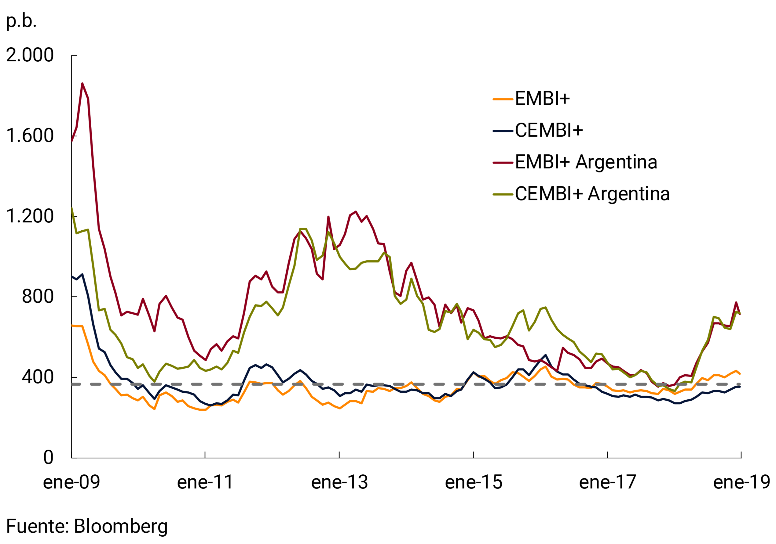
For Argentina, external credit conditions for foreign currency financing deteriorated compared to the third quarter. Argentina’s sovereign and corporate risk premiums thus rose to levels recorded in 2014, with widening of the relative gaps with respect to the rest of the emerging economies (see Figure 2.8), as is often the case in pre-election cycles. Also, the change in relative prices together with the performance of local economic activity led to higher levels of public and external debt in terms of GDP measured in dollars. In any case, together with the implementation of the new monetary program, the Argentine economy is heading towards a significant reduction in the twin deficits (current account and fiscal). In this way, correcting macroeconomic imbalances in terms of flows would contribute to economic growth based on more sustainable fundamentals.
In this context, the Argentine government prioritized the strategy of sovereign financing of multilateral origin, privileging placements in the local debt market, especially in national currency (capitalizable Treasury Bills and Treasury Bills indexed by inflation). In the last auctions, the interest rates on these bills were reduced. In addition, the refinancing rates of the maturities (roll over) of short-term bills were at levels even higher than those foreseen in the financing agreement with the International Monetary Fund (IMF). In the last agreement with this organization, the National Government obtained sufficient official financing so that it did not have the obligation to access financing in international markets practically until 2020. In the fourth quarter of 2018, there were no bond placements in the international markets by companies with local public offerings.
Figure 2.9 | Emerging Markets. Capital flows
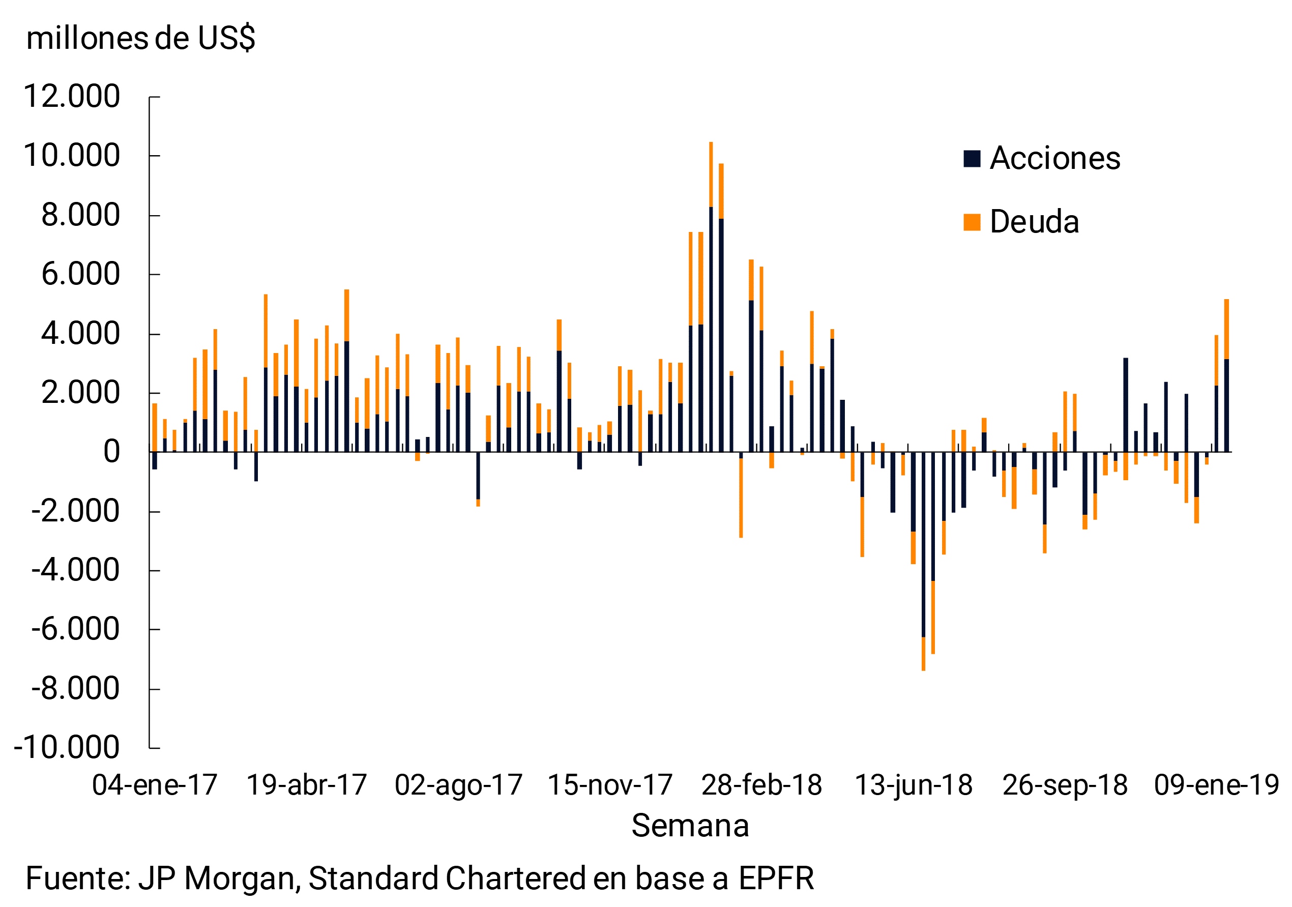
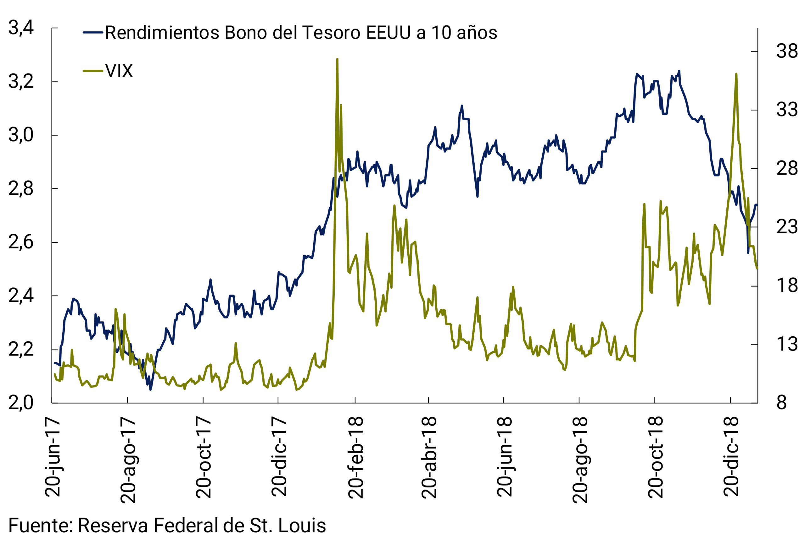
Recently, the depreciation of emerging market currencies has stopped, with a slight tendency to appreciate at the margin, along with a net inflow of capital into these markets (see Figure 2.9). In addition, the tightening of monetary conditions in the United States is also starting to ease. As already mentioned, fewer (or even none) increases in the Fed’s monetary policy rate are expected. In addition, the interest rate on the U.S. 10-year treasury note began to decline after the peak in early November (see Figure 2.10). This is why much of the financial outlook for 2019 will be influenced by whether this change in trend is maintained or only temporary. Finally, December saw a marked increase in financial market volatility (see Figure 2.8), linked in part to the performance of technology stocks.
Figure 2.10 | Financial market indicators
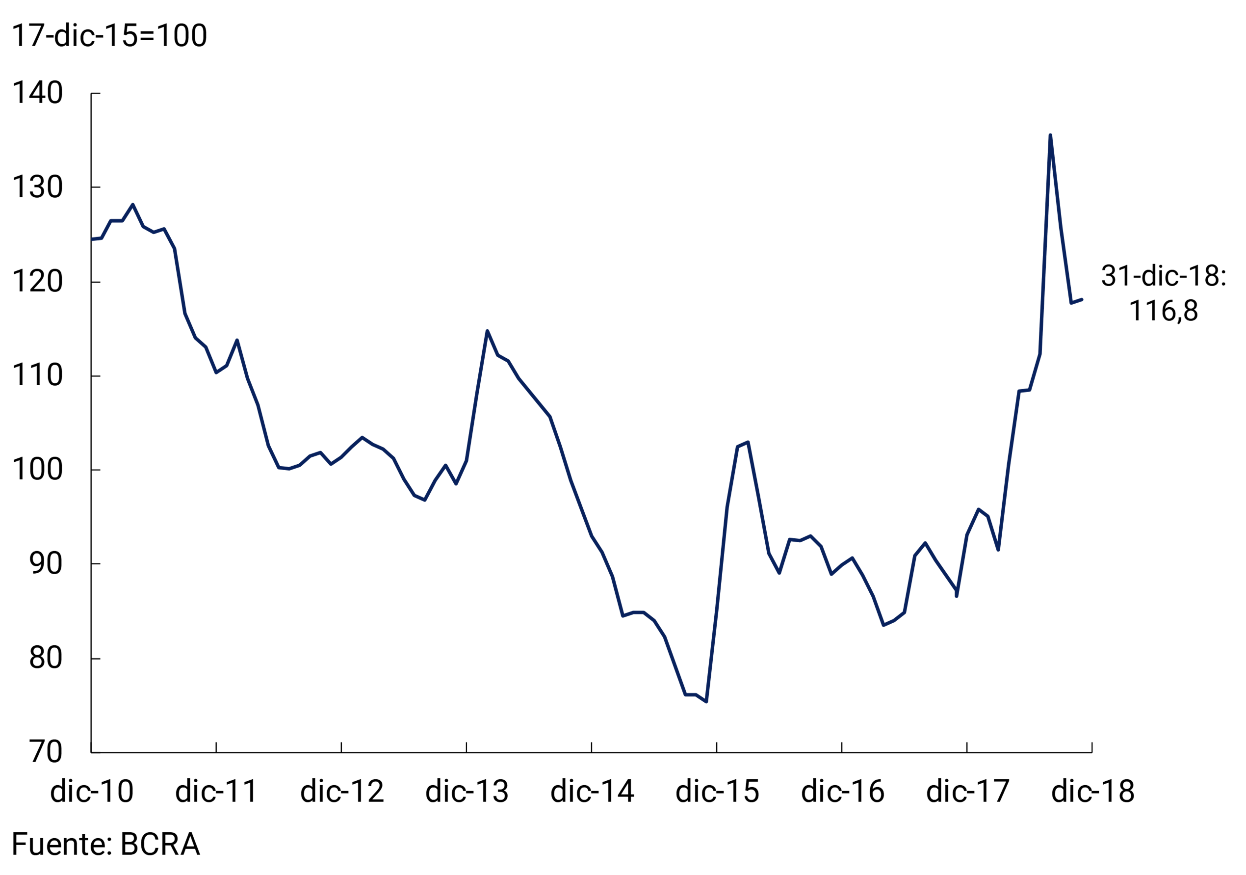
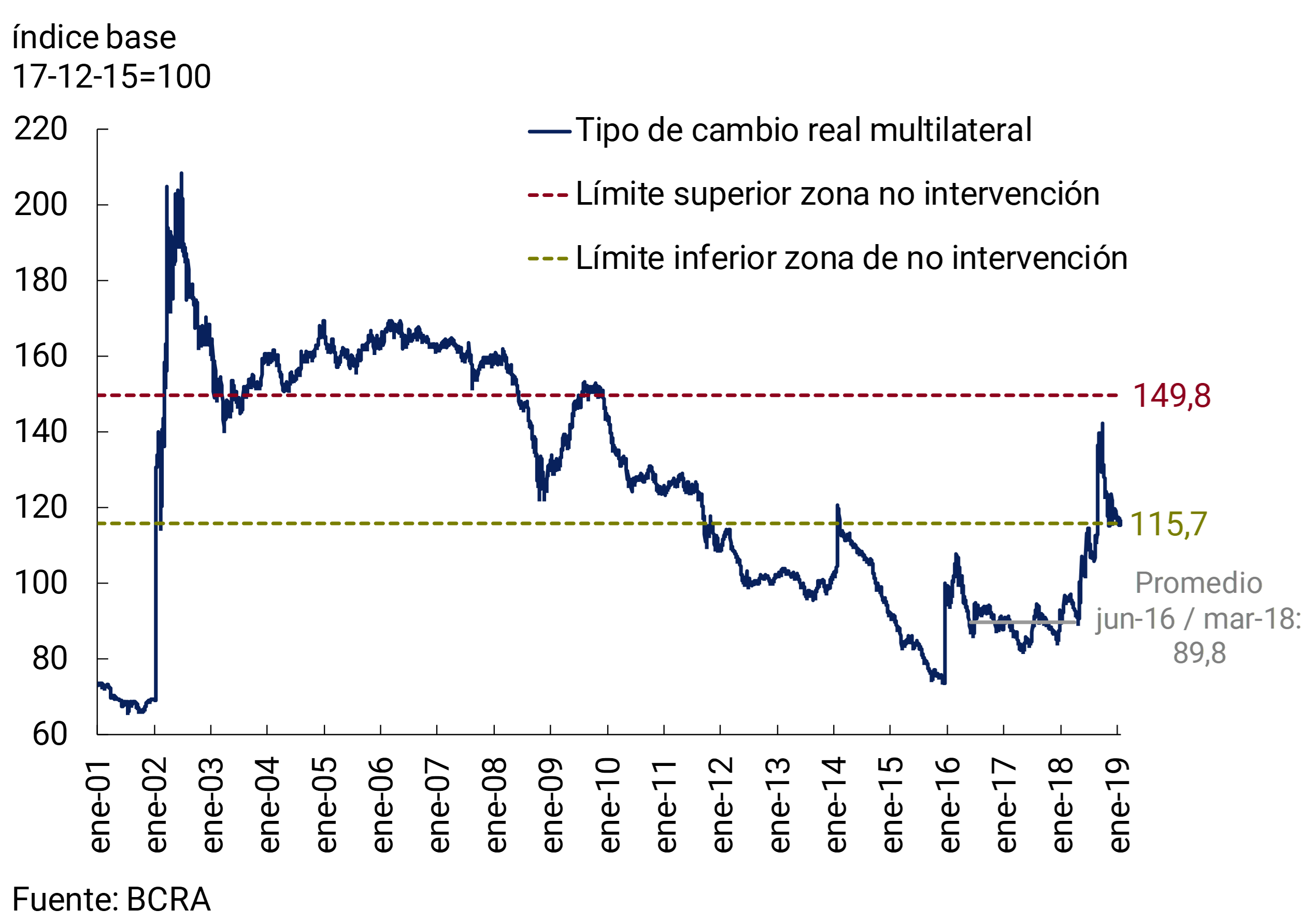
In the fourth quarter, the Multilateral Real Exchange Rate Index (ITCRM) rose 1.5% on average compared to the third quarter (see Figure 2.11), mainly due to a nominal depreciation of the peso against the dollar partially offset by local inflation. However, throughout the quarter (end to end) there was a real appreciation of the Argentine peso of 17%. Thus, in December, the ITCRM was around the levels recorded in 2010, when the trade balance registered a surplus of close to 3% of GDP.
Figure 2.11 | Multilateral Real Exchange Rate
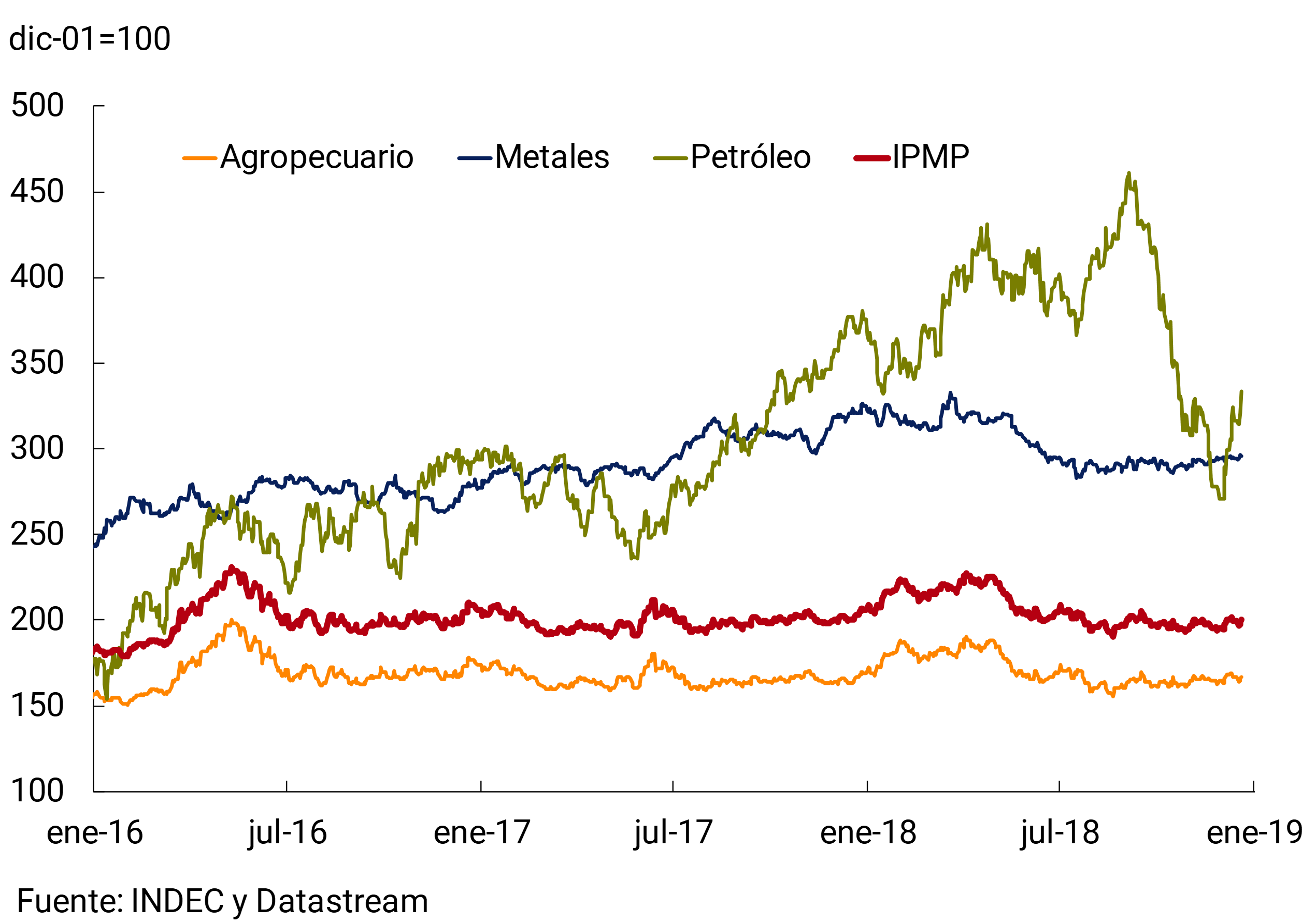
On the other hand, international commodity prices measured in dollars remained relatively stable in the fourth quarter of 2018, implying values that at the margin are approximately 2.7% below the levels of the same period of the previous year (see Figure 2.12). Because the Argentine economy is a net importer of energy and fuels, the abrupt fall in the international price of oil from the highest levels of recent years constitutes a factor in improving the terms of trade.
Figure 2.12 | International commodity prices
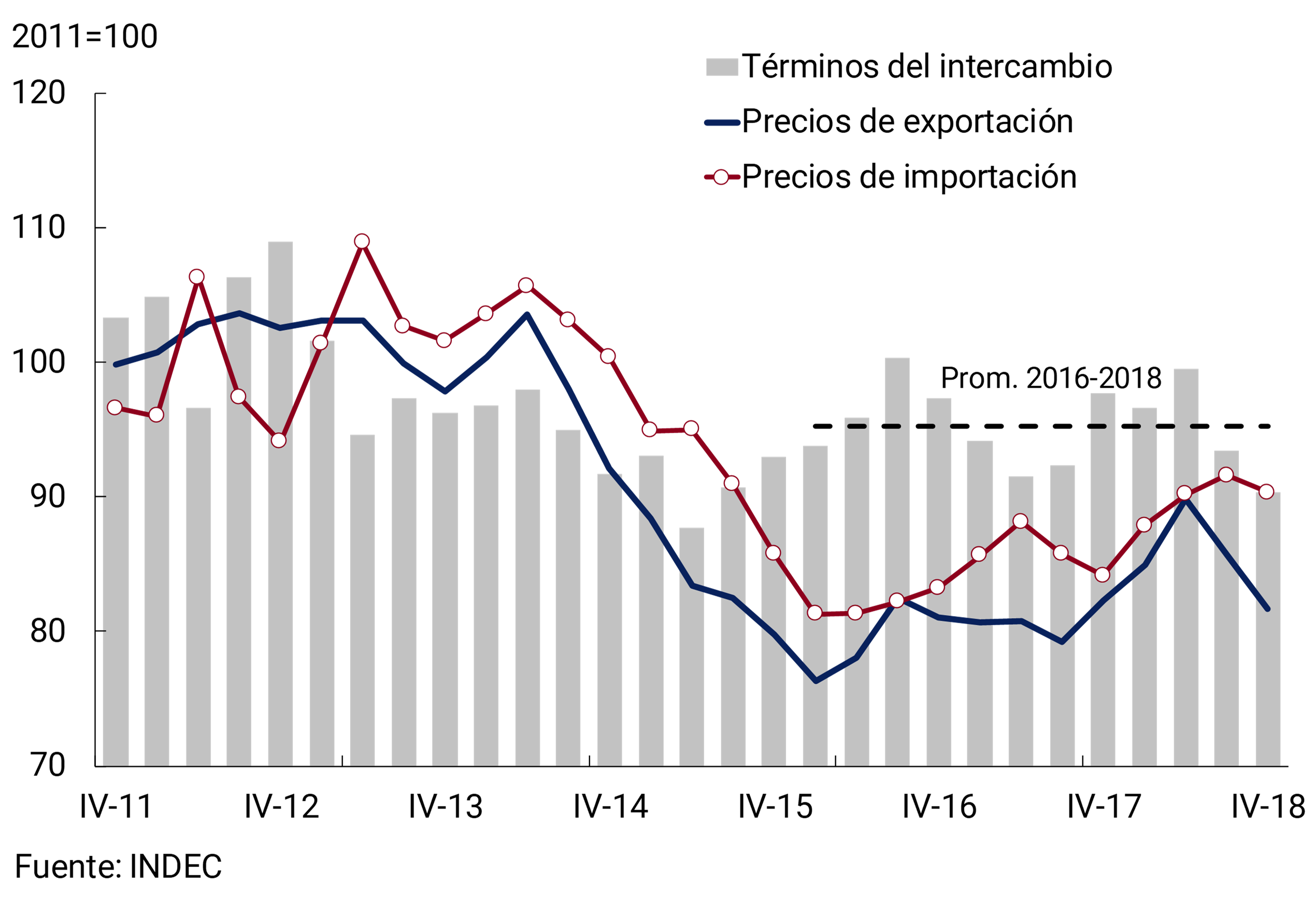
In any case, the terms of trade (ratio between the prices of Argentine exports and imports) fell 3.3% in the last quarter, as a result of a fall in the price of exports greater than that of import prices (see Figure 2.13). This evolution in export prices was influenced by the decline in the prices of agricultural products.
Figure 2.13 | Terms of Exchange
In summary, since the last IPOM, international financial conditions have had a slight improvement in the margin, although they continue to be markedly less favorable than those in force until 2017 (inclusive). On the other hand, the level of activity of our main trading partners is expected to perform well (mainly due to Brazil). All this would configure a mixed external scenario for Argentina. The main risks of this scenario are that the tightening of international financial conditions will regain momentum, a deepening of protectionist measures6, and that a deterioration in the level of global activity will take place.
3. Economic activity
The economy continued to contract during the fourth quarter of the year after the fall experienced in the previous two quarters. In the third quarter, the “non-agricultural” product deepened its contraction in line with the adverse scenario foreseen in the previous IPOM in a context of renewed financial and exchange rate tensions. The agricultural sector recovered after the drought that affected the soybean and corn harvest, attenuating the fall in GDP. Consumption and investment, both public and private, showed declines that continued in the last quarter of 2018, while the positive contributions of net exports gradually began to be noticed, in a framework of fiscal consolidation. As of December, the application of a set of income policies aimed at compensating lower-income sectors together with the reopening of parity agreements in several branches of activity made it possible to shore up consumption.
The monetary plan for strict control of the monetary base, together with the announcement of the acceleration of fiscal convergence, made it possible to normalize the situation in the foreign exchange market, gradually reduce inflationary records and begin to recover a nominal anchor for expectations. The possibility of providing a horizon of increasing nominal certainty is one of the main contributions of the BCRA to achieving a stable macroeconomic environment that favors growth.
For 2019, it is expected that this combination of monetary and fiscal policies will allow a return to the path of declining inflation and enable a gradual recovery of the level of activity. This view is shared by REM analysts who expect activity to reach a floor in the first quarter of the year and, from there, to enter a cyclical phase of reactivation. A more competitive real exchange rate will boost activity in tradable sectors and, together with the reduction of the fiscal deficit, is contributing to a rapid reversal of the current account imbalance. The correction of these imbalances will reduce the vulnerabilities of the Argentine economy and will make it possible to start a stage of growth on a more sustainable basis.
3.1 Activity would reach a floor during the first quarter of 2019
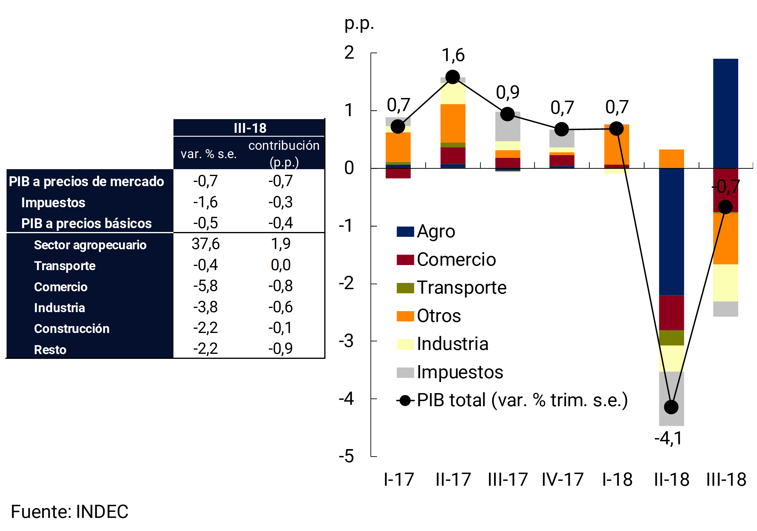
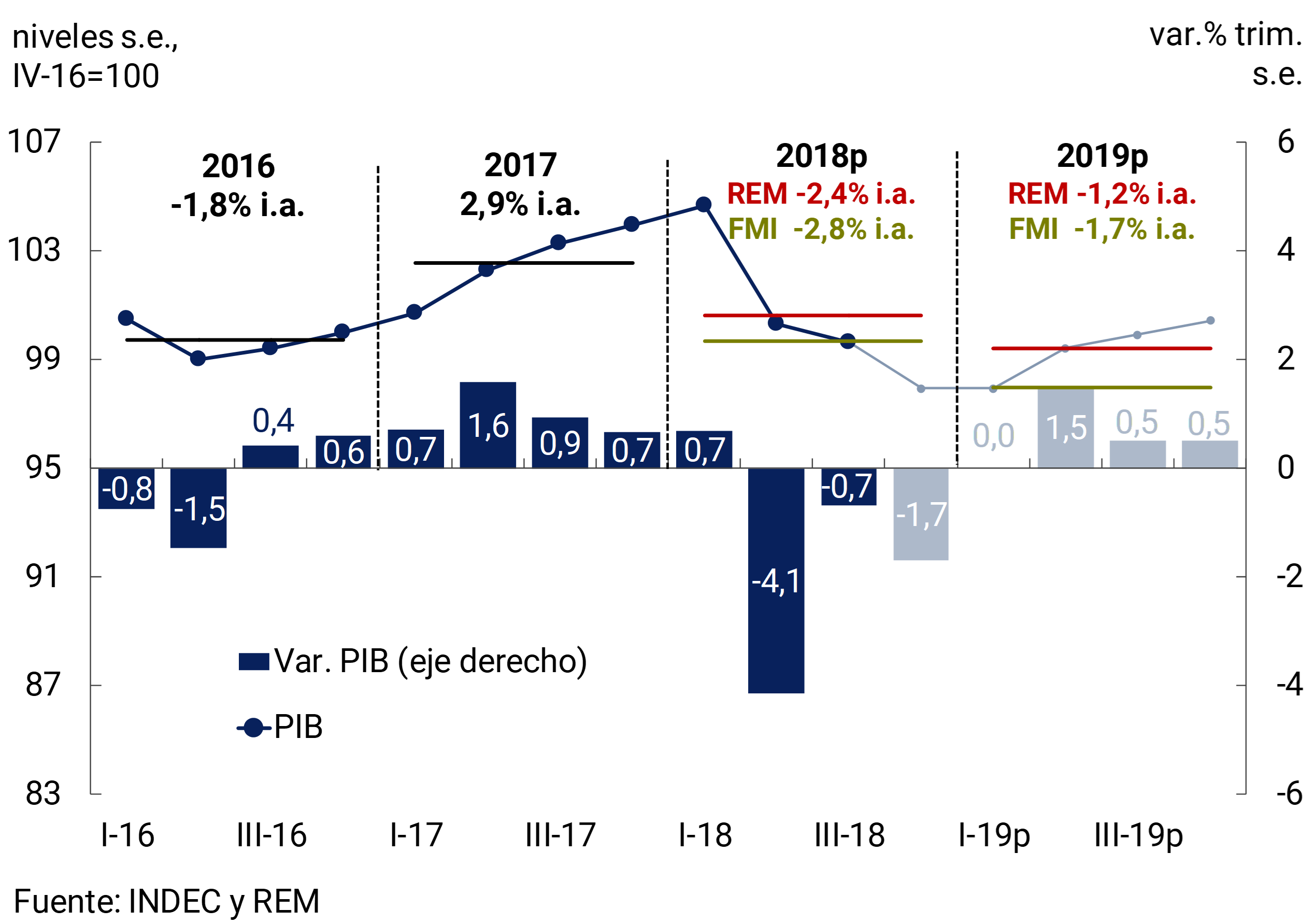
In a context of renewed financial and exchange rate tensions and a sharp increase in uncertainty, economic activity contracted in the third quarter of the year (-0.7% s.e. and -3.5% y.o.y.), after the sharp fall experienced in the second quarter (-4.1% s.e. and -4% y.o.y.).
Activity indicators anticipate a further fall in the fourth quarter. INDEC’s Monthly Estimator of Economic Activity (EMAE) registered a 0.9% monthly increase s.e. in October, but would contract again in November due to the weak performance of industry and construction. The O.J. Ferreres General Activity Index also increased in October (0.5% month-on-month s.e.) and fell again in November (-1.2% s.e.; see Figure 3.1). The latest Contemporary GDP Prediction of the BCRA (PCP-BCRA) for the fourth quarter indicates a fall of 2.3% quarter-on-quarter s.e., while the median of the REM shows a decrease of 1.7% quarter-on-quarter s.e.
Figure 3.1 | Evolution of economic activity

Although during the last quarter of 2018 the economy continued to contract—due to the marked reduction in revenues in real terms and the shortening of decision-making horizons due to uncertainty—the positive contribution of the external sector gradually began to become evident. At the same time, as of December, the implementation of a set of income policies aimed at households with a high propensity to consume together with the reopening of parity agreements in several branches made it possible to shore up consumption, leaving a higher level for the beginning of the first quarter of 2019.
In line with this, the Leading Indicator of Activity (ILA-BCRA) for the month of December showed the first monthly growth after nine consecutive months of decline, the diffusion of growth improved marginally and the depth of the accumulated fall in six months was reduced. This improvement in the ILA is not enough to say that the recessionary phase of activity has come to an end, so new signals should accumulate in the coming months to ensure the existence of a pivot point for activity. The analysts participating in the REM estimate that during the first quarter the GDP will reach a minimum and from there resume a trajectory of gradual growth.
3.1.1 Positive contributions from net exports are beginning to be noticed
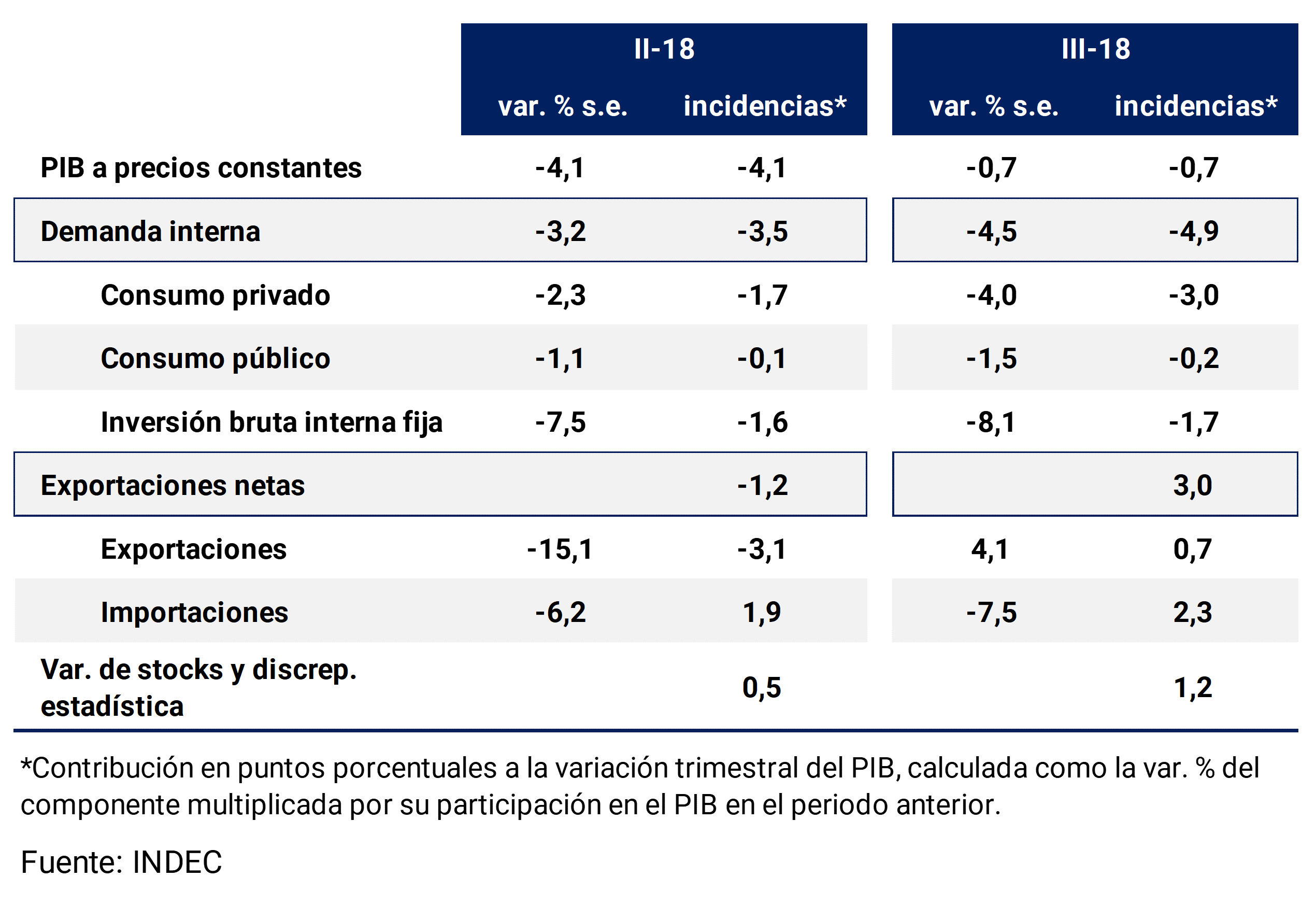
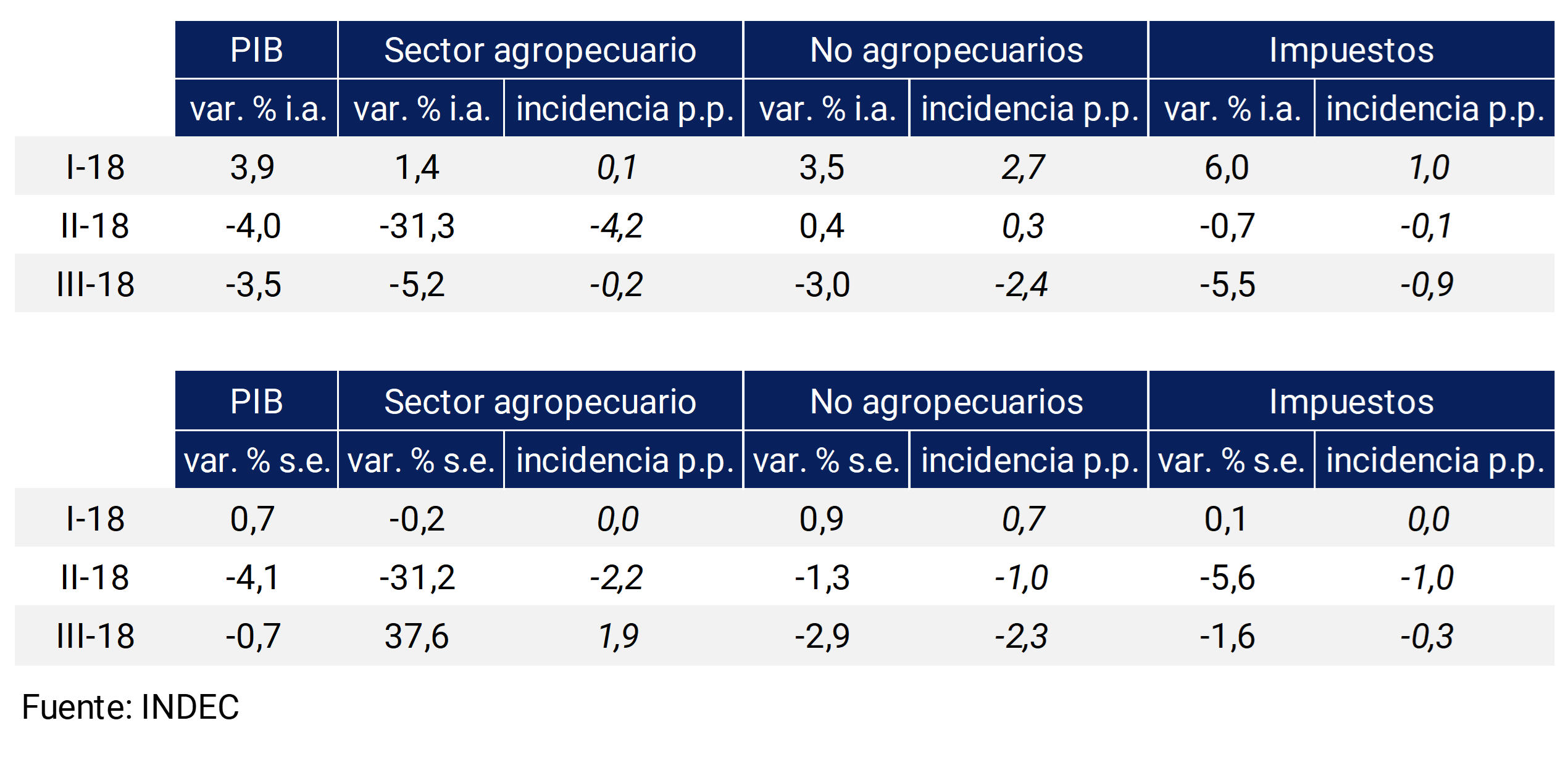
As anticipated in the previous IPOM, in the third quarter exports of goods and services began to recover (+4.1% quarter-on-quarter s.e.) while imports deepened the fall already observed in the previous quarter (-7.5% quarter-on-quarter s.e.). As a result, the external sector contributed positively with 3 percentage points (p.p.) to the quarterly variation in GDP and it is estimated that the contribution was even greater in the last quarter of last year, partially offsetting the marked contraction in domestic demand (see Table 3.1).
Table 3.1 | Quarterly change in GDP and contributions of its components
In the last quarter of 2018, the performance observed in exports and imports was accentuated. Exported quantities of goods grew 15.8% s.e. compared to the previous quarter (+11.2% y.o.y.), while imported volumes fell 14.7% s.e. (-28.9% y.o.y.; see Figure 3.2). Thus, the contribution of net exports of goods and services to seasonally adjusted quarterly output growth is expected to have been strongly positive, exceeding 4 p.p., reflecting the marked correction experienced by the external sector.
Figure 3.2 | Exports and Imports of goods and services

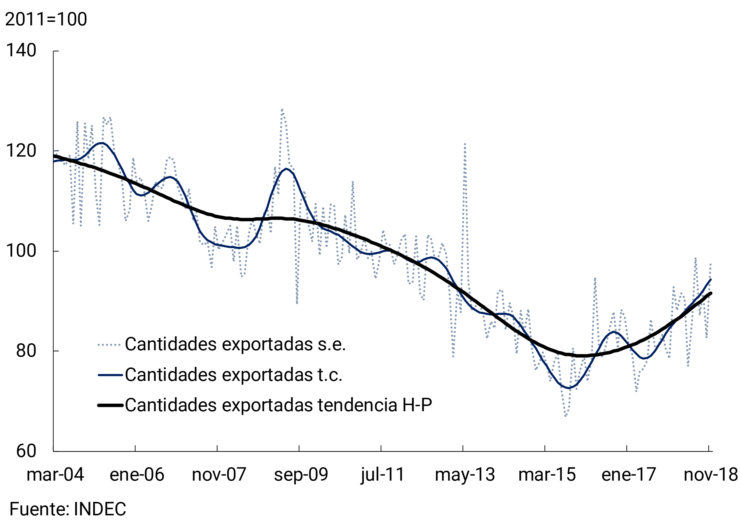
In the fourth quarter, non-agricultural exports sustained the growth they have exhibited since the beginning of 2016, when the downward trend they registered for more than ten years was reversed (see Figure 3.3). On the margin, this good performance of non-agricultural exports was compounded by the rebound in soybean shipments to China in the context of its trade disputes with the United States.
Figure 3.3 | Exported quantities of goods (excluding major grains and derivatives)
From June onwards, export growth was strong and widespread. The share of sectors whose exports grew from the previous month remained above 50%, the longest expansion since 2009. Among the sectors with the highest growth rates are oilseeds, fuels, industrial manufactures (rubber, paper, metals, and plastics), and agricultural manufactures (fish and seafood, meat, and plant extracts; see Figure 3.4).
Figure 3.4 | Exported quantities of goods
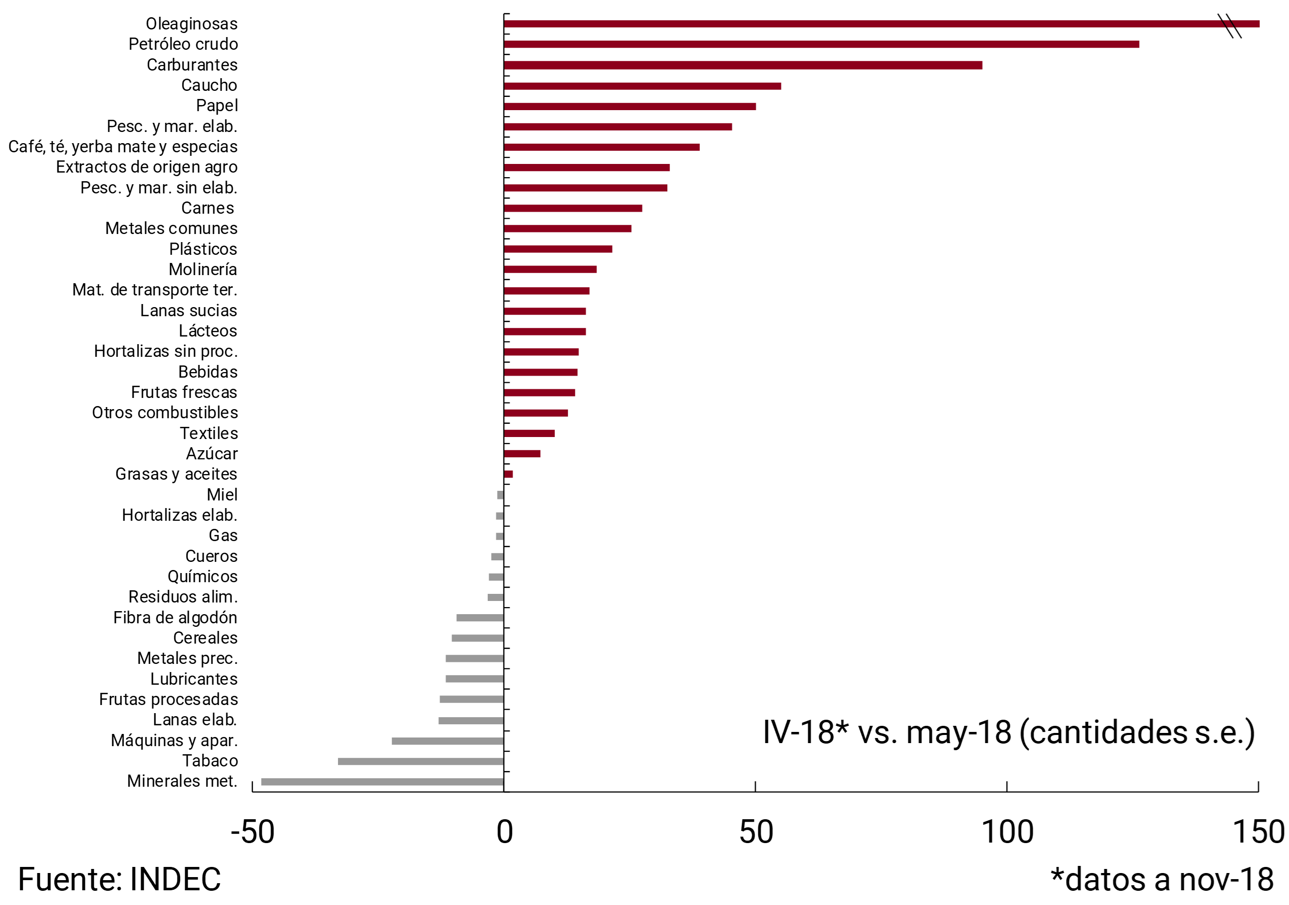
A number of factors influenced the favorable performance of foreign sales: the improvement in the real exchange rate, greater external demand—particularly from Brazil and China—and the increase in unconventional hydrocarbon production in Vaca Muerta. It should be noted that this increase in exports occurred in a context of reduced transaction costs brought about by a battery of measures aimed at eliminating and/or facilitating the procedures necessary to export, as well as a policy of opening new markets.
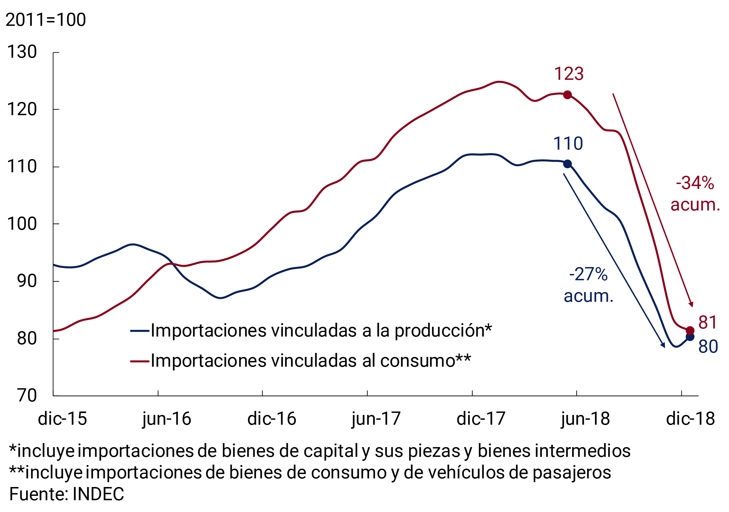
As for imports, the contraction continued during the fourth quarter. After 3 consecutive quarters of declines, imported quantities were at the lowest levels in the last 4 years in December. In line with the decline in domestic absorption, both consumption-related and investment-related imports declined (see Figure 3.5). This reduction in imports was widespread. In the October-November period, only 2 of 19 groups of goods showed increases compared to the previous quarter (vegetable inputs and mineral inputs). The sharpest falls were recorded in imports of industrial transport equipment, vehicles for the transport of people, non-durable consumer goods and textile fibers (-29% s.e., -25% s.e., -21% s.e. and 18% s.e., respectively).
Figure 3.5 | Imported quantities of goods (e.g. mobile avg. 3 months)
The external balance of services also showed an adjustment in the third quarter of 2018, which was consolidated in the last quarter of the year. Due to its importance within the balance of services, the cut in the deficit for tourism stands out, in the second half of 2018 it was around US$ 1,800 million, approximately half of that recorded in the same period of 2017.
As a result of the aforementioned correction in trade flows in goods and services, during the second half of the year there was a significant reduction in the current account deficit, one of the vulnerabilities exhibited by the Argentine economy in the last period and which was at the origin of the episode of sudden halt in voluntary financing experienced from the second quarter of this year (see Box).
Box. The correction of the current account deficit
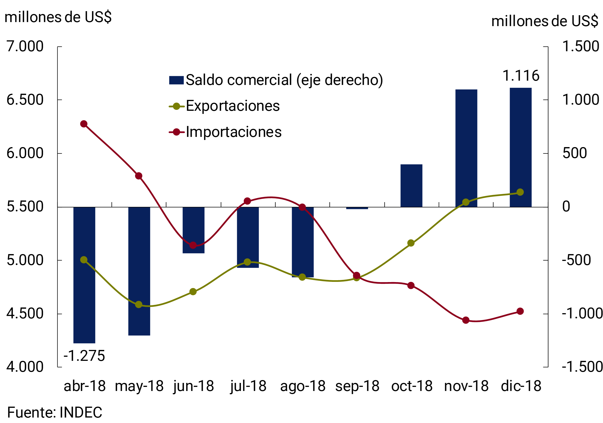
In the IPOM of October 2018, the estimate of a significant adjustment of the current account as of the third quarter of that year was anticipated, mainly as a result of the real depreciation of the peso and lower domestic absorption. Recent foreign trade data validated those expectations. The seasonally adjusted trade balance of goods went from a deficit of US$1,275 million in April to a surplus of US$1,116 million in December. The magnitude of this reversal – US$ 2,390 million in 8 months – is unprecedented if we take into account the information available over the last 26 years.
The adjustment in the trade balance was due to both a fall in imports and an increase in exports7 (see Figure 3.6).
Figure 3.6 | Foreign Trade of Goods (s.e.)
The correction in external flows was not limited to goods. In the third quarter of 2018, the deficit in the balance of services was reduced by US$ 544 million YoY, mainly due to lower expenditures due to outbound tourism. The advance data allow us to observe a deepening in the deficit cut in the fourth quarter.
The combination of a reversal in the trade balance of goods and a decline in the deficit in services results in a significant correction of the economy’s current account balance. Adjusting for seasonal factors, in annualized terms the current account balance in the fourth quarter would be around -1.2% of GDP, which implies a reduction in the deficit of 5.4% p.p. of GDP in just one quarter. Thus, in seasonally adjusted terms, the economy would have started 2019 with a current account deficit similar to the average of the last 13 years (see Figure 3.7).
Figure 3.7 | Current account and real exchange rate
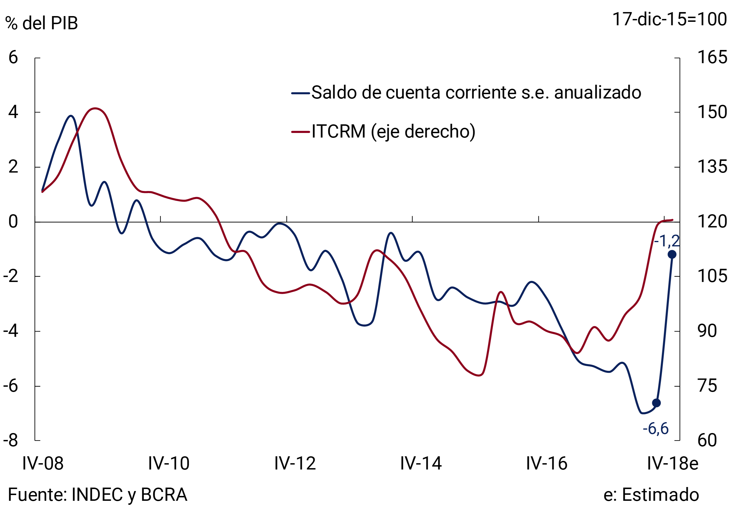
At the beginning of 2018, dependence on external savings was one of the main vulnerabilities of the economy. During the first half of that year, a series of external and internal shocks caused a change in market sentiment that implied a preference for foreign assets and a marked rise in the real exchange rate. From the second half of the year, external flows responded to the change in the macroeconomic scenario. The data suggest that a significant part of the adjustment to the new conditions has already materialized. After this correction, the economy will be able to resume a path of growth on more sustainable bases.
3.1.2 During the fourth quarter of 2018, the fall in domestic absorption continued, but in December some signs appeared that would point to a recovery in private consumption
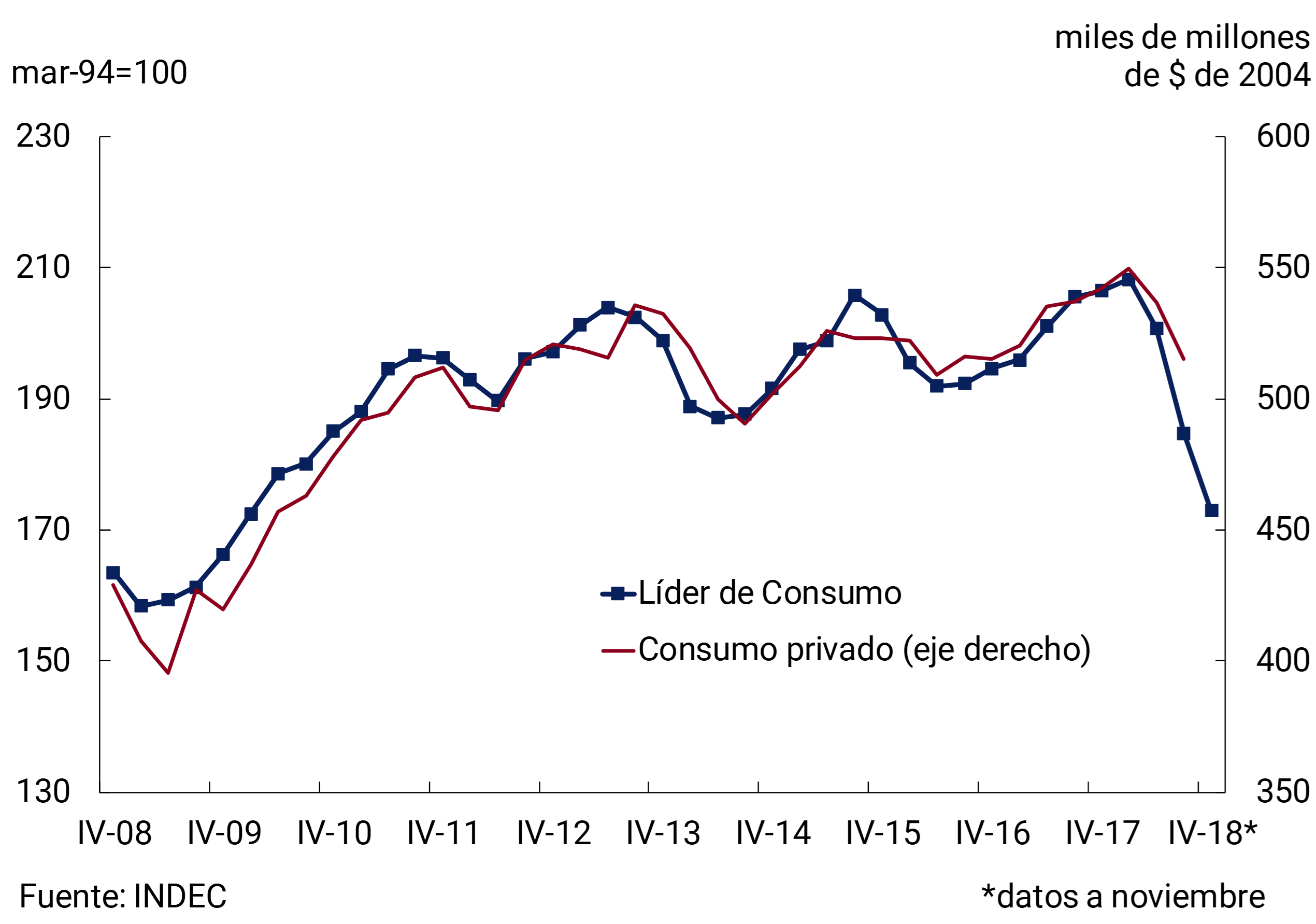
During the third quarter of 2018, private consumption deepened its decline (-4% s.e.; -4.5% y.o.y.), affected by the deterioration in real disposable income of households and the negative evolution of consumer expectations, in a context of renewed uncertainty and more restrictive credit conditions. With data from October and November, theBCRA’s Leading Indicator of Private Consumption 8 shows a new drop in consumption for the fourth quarter (see Figure 3.8).
Figure 3.8 | Level of private consumption
However, at the end of 2018, increases in the income of segments with a high propensity to consume were observed. A part of these increases were granted by the government while, due to the renegotiation of some parity agreements as of November, the salaries of the formal segment were raised. This in a context in which inflation in December (2.6% monthly) was the lowest since May 2018.
Among the extraordinary revenues in December, the granting of $1,500 as a reinforcement to family allowances per child for around 4 million beneficiaries9 stands out. Retirees and pensioners also received the quarterly update of salaries in December, when the previous year the adjustment was semi-annual and had occurred in September. Added to this were the year-end bonuses granted to provincial state employees (940,000 people for an average amount of $6,878), to the security forces, armed forces and other national state employees and the bonuses received by some formal employees in the private sector10. It is estimated that together all these additional revenues in December would have meant an increase equivalent to approximately 3 p.p. in average monthly private consumption at current prices.
Thus, although the quarterly average of seasonally adjusted private consumption would continue to contract during the last quarter of 2018, the month of December could leave a higher level for the first quarter of this year, in which activity is expected to reach a floor. In this sense, the first indicators for December show some positive signs regarding the behavior of private consumption. In December, there was growth in both car sales in the domestic market (10.2% monthly s.e.) and imports of consumer goods (9.2% s.e.), in a context of improved consumer confidence at the national level (12.1% in December; ICC-UTDT)11.
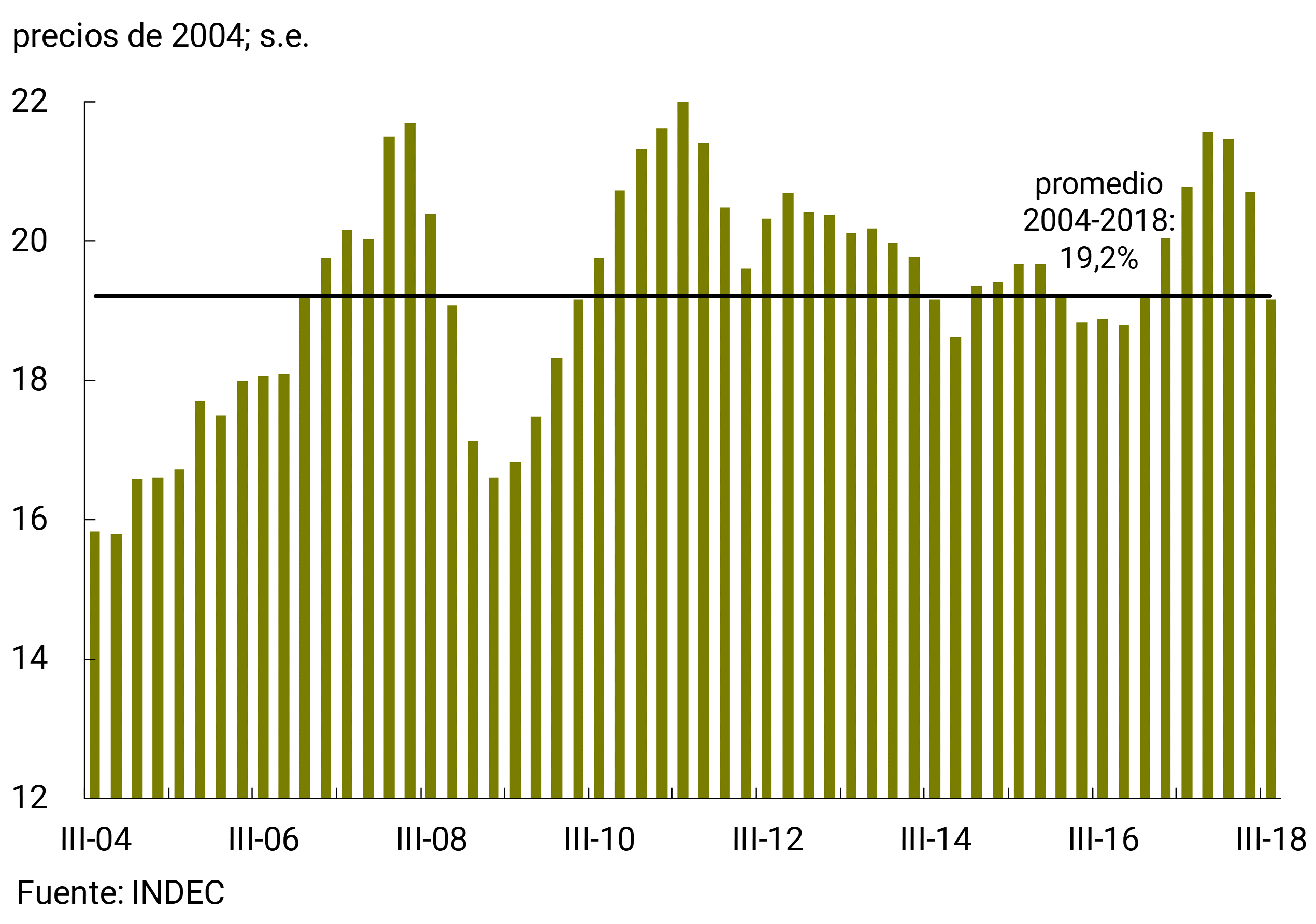
Investment reflected the increase in the relative price of capital goods, the deterioration of domestic financial conditions and the unfavorable outlook for the evolution of domestic demand, showing a contraction in the third quarter of 8.1% s.e. (-11.2% y.o.y.) after falling 7.5% s.e. in the second quarter (+2.9% y.o.y.). The investment-to-GDP ratio stood at 19.2% in seasonally adjusted terms in the third quarter of 2018, reducing by 2.4 p.p. from the last peak in the fourth quarter of 2017. In historical perspective, this level of investment is considerably higher than the minimum of 16.6% reached during the 2009 crisis and is equal to the average for the series beginning in 2004 (see Figure 3.9).
Figure 3.9 | Gross fixed capital formation as a percentage of GDP
Among the components of gross investment, during the third quarter of 2018 the reduction in durable equipment stood out (-15.5% quarter-on-quarter and 18.5% y.o.y.), mainly explained by the sharp contraction in imported quantities of transport material (-32.1% quarter-on-quarter and 36% y.o.y.). Construction also fell (-2.6% QoQ/Y and -1.5% YoY).
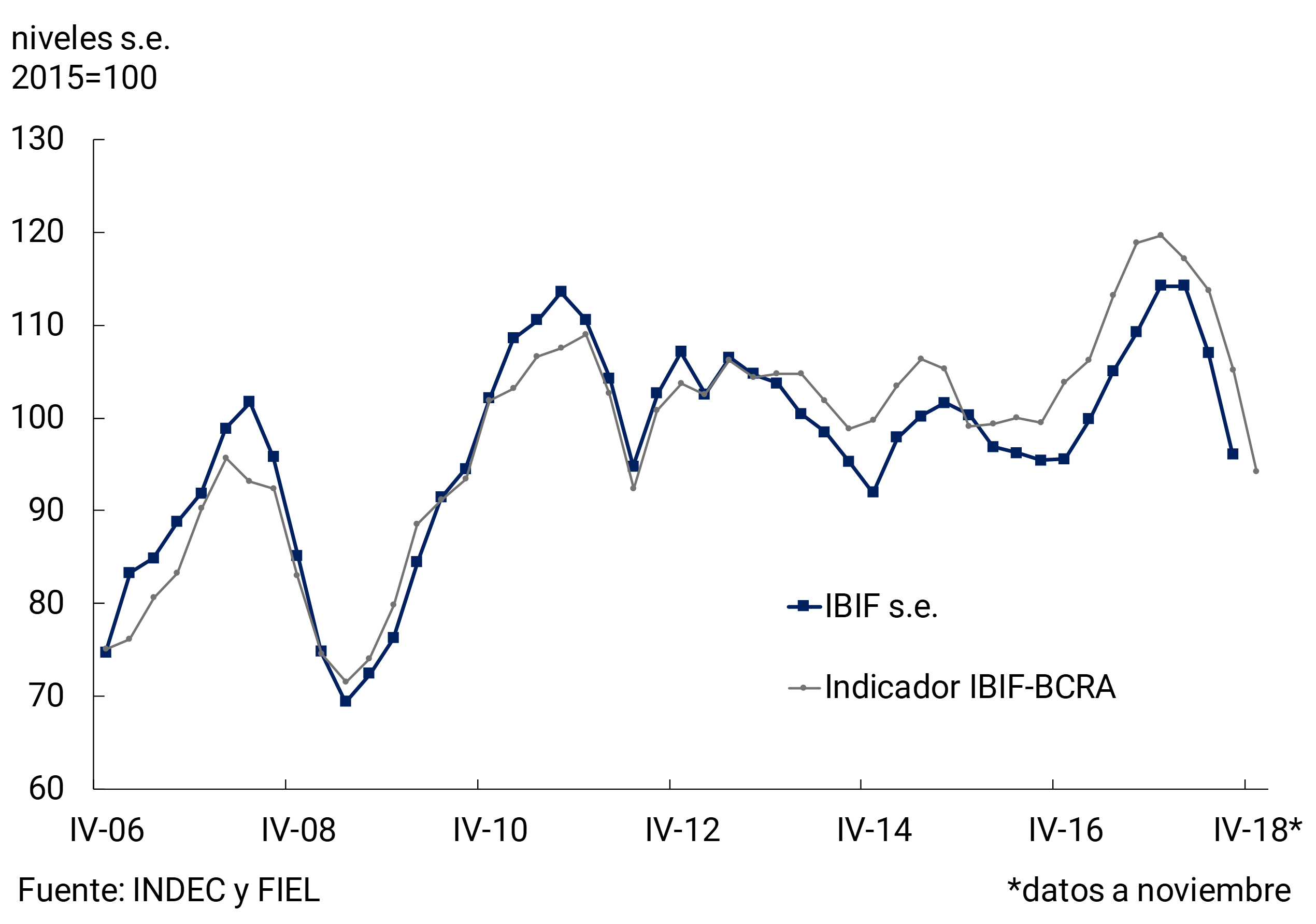
Partial indicators indicate that in the fourth quarter the fall in investment was accentuated, due to the reduction in spending on durable equipment and the lower activity of both public and private construction. With data up to November, the IBIF-BCRA12 indicator shows a fall of 10.4% s.e. compared to the previous quarter (see Chart 3.10).
Figure 3.10 | Investment evolution
In the last months of 2018 and the beginning of 2019, macroeconomic uncertainty was reduced—in a relatively more favorable international context—and lower lending rates were verified in the financial system, which allowed debt and trust issuances to slowly return to the domestic capital market.
3.1.3 In the last quarter of 2018, the rate of decline in non-agricultural output was maintained, while some activities showed signs of the beginning of the reactivation that is projected for the beginning of 2019
Table 3.2 | Sectoral evolution of GDP
The official data confirmed the forecast in the IPOM for October 2018 regarding the evolution of activity in the third quarter. The decline in the non-agricultural sectors accelerated, while the agricultural sector showed a strong rebound after the drought, which partially offset the fall in the rest of the economy (see Table 3.2).
The contraction in activity in the third quarter was highly widespread: 13 of the 16 sectors of GDP fell in seasonally adjusted terms with respect to the second, with agriculture, fishing and domestic service in private households being the only exceptions. Strong contractions were seen in industry and construction, while trade was the services sector most affected by weak domestic demand. The direct contribution of the rebound in agriculture to seasonally adjusted growth was approximately 1.9 p.p., also contributing to the reduction of the rate of contraction in associated sectors such as transport13 (see Figure 3.11).
During the fourth quarter of 2018, the contraction in domestic demand continued to negatively affect activity in the main sectors. Non-agricultural output would have fallen at a rate similar to that of the previous quarter while agriculture would have remained relatively stable, leaving behind the statistical rebound after the drought. Thus, the seasonally adjusted quarterly fall in total GDP would have been greater in the fourth quarter than in the third (-1.7% according to the median of the REM, while the latest available estimate of the PCP-BCRA indicates a somewhat larger quarterly contraction, in the order of -2.3%).
Figure 3.11 | Sectoral evolution of activity
Different official and private indicators showed a sharp contraction in the main activities producing non-agricultural goods in the fourth quarter of 2018. The negative effect of the fall in domestic demand could not be offset by the increase in exports. With data up to November, it is estimated that the fall in the manufacturing sector would have been similar or slightly lower than that of the third quarter, while construction accelerated the pace of contraction. According to preliminary data from the EMAE and projections for November and December 2018 based on the evolution of the indicator in the drought episodes in 2009 and 2012, it can be estimated that the output of the agricultural sector would have remained stable in the fourth quarter in seasonally adjusted terms with respect to the third quarter (see Figure 3.12).
Figure 3.12 | Main sectors producing goods

According to the EMAE of October 2018, it is likely that the quarterly (seasonally adjusted) decline in the activity of the service provider sectors slowed down during the fourth quarter. Although data for November and December are not available, the statistical carry-over from October for the fourth quarter suggests a slowdown in the fall compared to the strong negative rates evidenced in the third. Activities related to tourism, such as hotels and restaurants, and transportation have begun to recover, benefiting from the improvement in the real exchange rate. Financial intermediation, affected by lower demand for loans, was the only services sector that accelerated its contraction compared to that evidenced in the third quarter (see Figure 3.13).
Figure 3.13 | Activity in service-producing sectors
Supply-side sectors can be classified into at least four groups according to their performance since the beginning of the recession and their medium-term prospects.
A first group is made up of activities directly and indirectly affected by the drought (agricultural sector, transport, agricultural machinery, manufacture of transport equipment, among others). These sectors have begun to recover since the third quarter and this dynamic is expected to continue in the face of favorable harvest projections for 201914.
In the second group are a set of activities driven by economic policies adopted since the beginning of the current administration, such as the opening of new international markets, deregulation and incentives for private investment. These sectors include beef and pork slaughter, unconventional crude oil and gas extraction, iron and steel production, non-refrigerated dairy production, and commercial airline activity. Since most of these activities are export-oriented, their favourable trend is expected to consolidate as new markets continue to open up and the improvement in the real exchange rate translates into increased competitiveness and profitability.
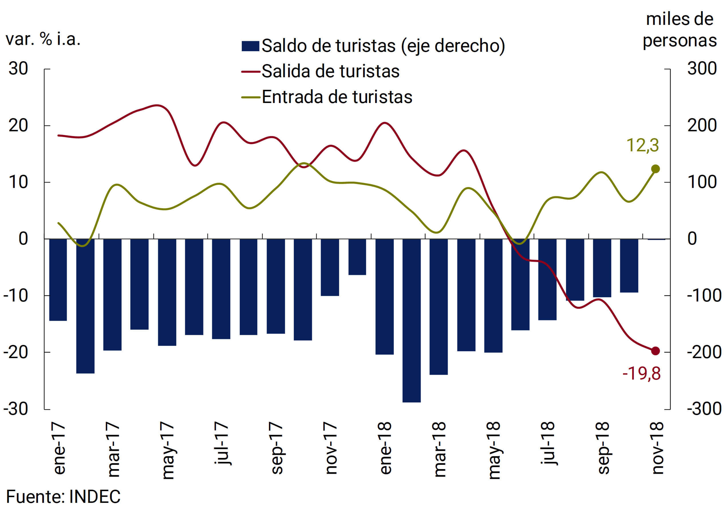
Another group is made up of activities that are oriented to the production of tradables and that, although they were affected by the contraction of the domestic market, could begin a growth process. These favorable prospects are based on the improvement in profitability from the correction of the real exchange rate evidenced in 2018 and the greater external demand from Brazil. The first signs in this regard can be seen in inbound tourism. The data up to November 2018 show a consolidation of the positive trend in the number of foreign tourists visiting Argentina and a negative trend in the number of residents who are tourists outside the country. This favorable dynamics of tourism impacts related activities such as transportation, hotels, restaurants and some items of retail trade. The preliminary EMAE data available as of October 2018 are in line with this forecast (see Figure 3.14).
Figure 3.14 | International tourism
Finally, the group of sectors mainly oriented to the domestic market—the one with the greatest weight in GDP—was the most affected by the fall in the real wage bill, the increase in real interest rates, and the uncertainty associated with exchange rate instability during 2018. The outlook is that these activities will begin to gradually recover from historically low levels during the first quarter of 2019, as domestic consumption finds a floor and begins to reactivate in a context of greater financial stability and nominal certainty.
3.1.4 The prolongation of the contractionary phase of activity was reflected in a slight deterioration in labour market conditions
During the third quarter of 2018, registered employment maintained the slightly declining trend. This decrease in formal employment was explained by the fall in private salaried employment in a context in which the levels of private self-employment and public employment are sustained. (see Figures 3.15 and 3.16).
Figure 3.15 | Total registered employment (e.g.; excluding the social monotax)
Figure 3.16 | Registered employment by category (e.g.; excluding the social monotax)
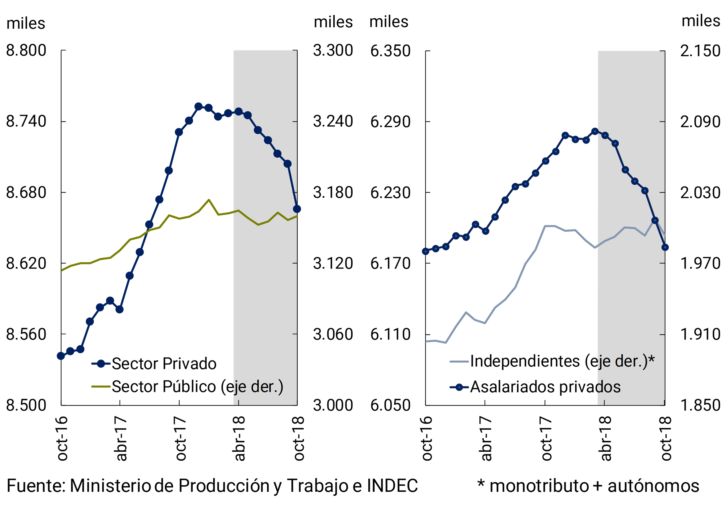
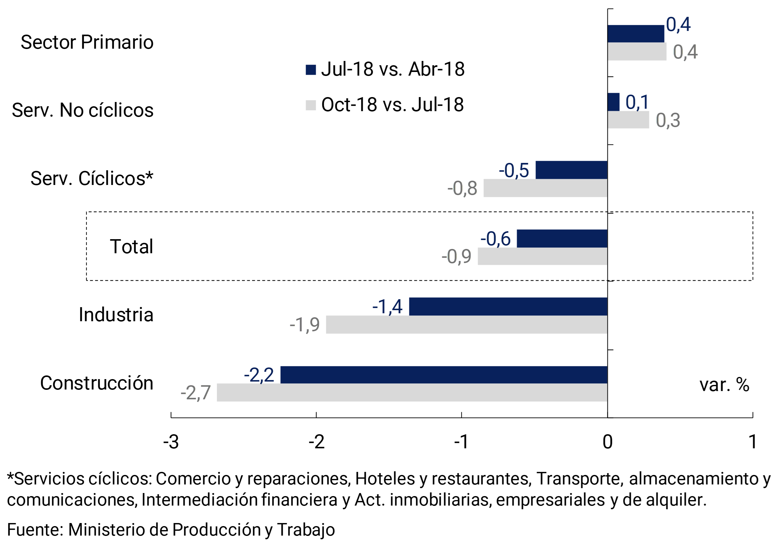
Salaried private employment accentuated its fall due to the behavior of sectors associated with the cycle during the period Jul-18/Oct-18. The main falls in employment were registered in the areas of construction, industry and cyclical services, such as transportation, commerce and hotels and restaurants. In contrast, jobs in the primary sector and in the rest of the services increased slightly. (see Figure 3.17).
Figure 3.17 | Cumulative change in private salaried employment by sector (s.e.)
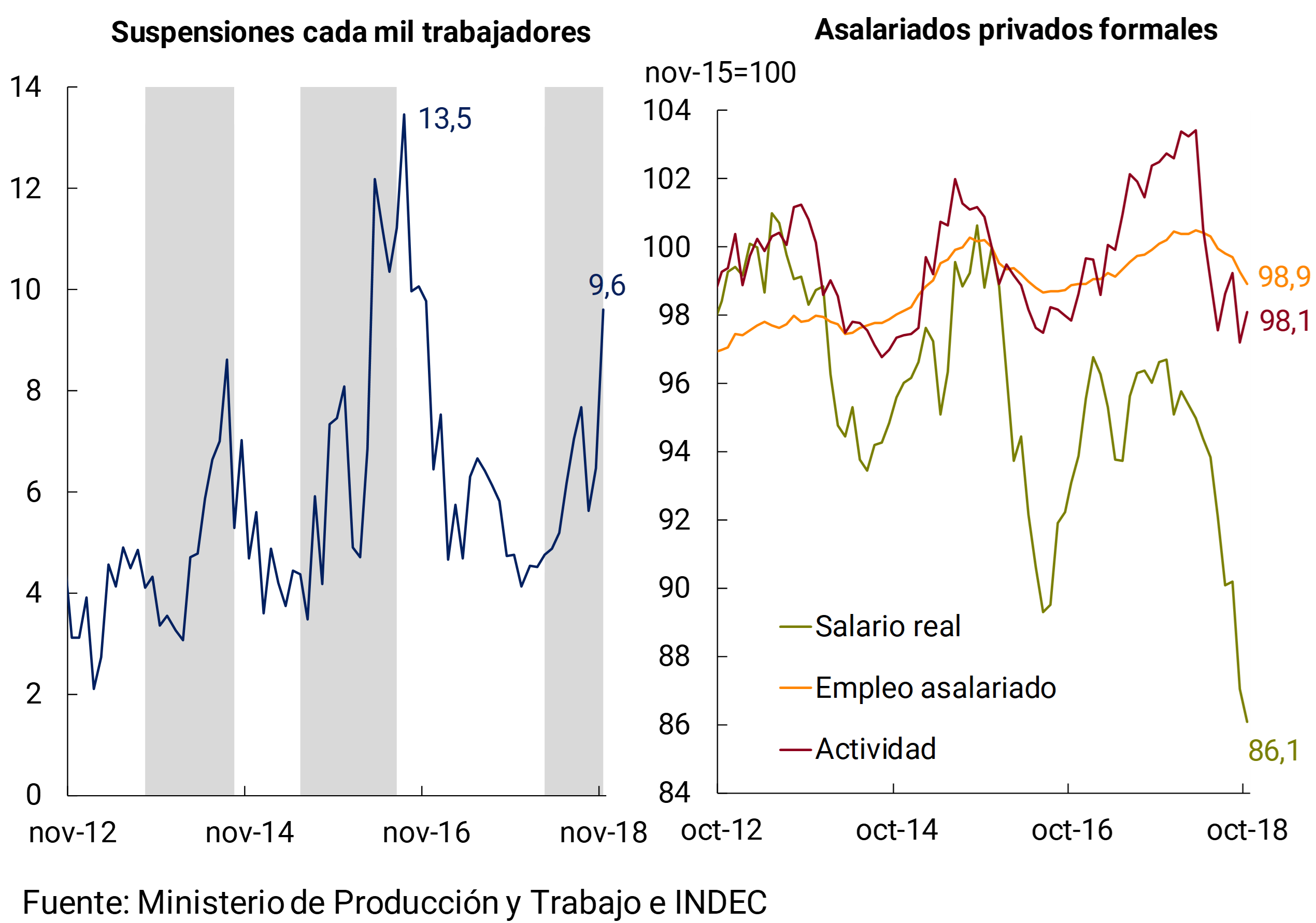
In the face of the significant contraction in domestic demand during the second half of 2018, so far companies have responded in part by underutilizing the labor factor – by showing a growing number of suspensions and reduction in hours worked – moderating staffing reductions (data from the Survey of Labor Indicators of the Ministry of Production and Labor). This business behavior – which allowed the adjustment of the quantities demanded of the labor factor at the aggregate level to have been less than the contraction of economic activity during the period – was facilitated by the adjustment of real wages observed since the beginning of the recession. In addition, the flexibility shown by the exchange rate in Argentina reinforces these trends. The depreciation of the local currency that resulted in the increase in wages increased the external competitiveness of the economy, thus reducing the incentives for an adjustment in the number of jobs (see Figure 3.18 and Section 2. of Unit Labor Cost).
Figure 3.18 | Suspensions and Real Salary
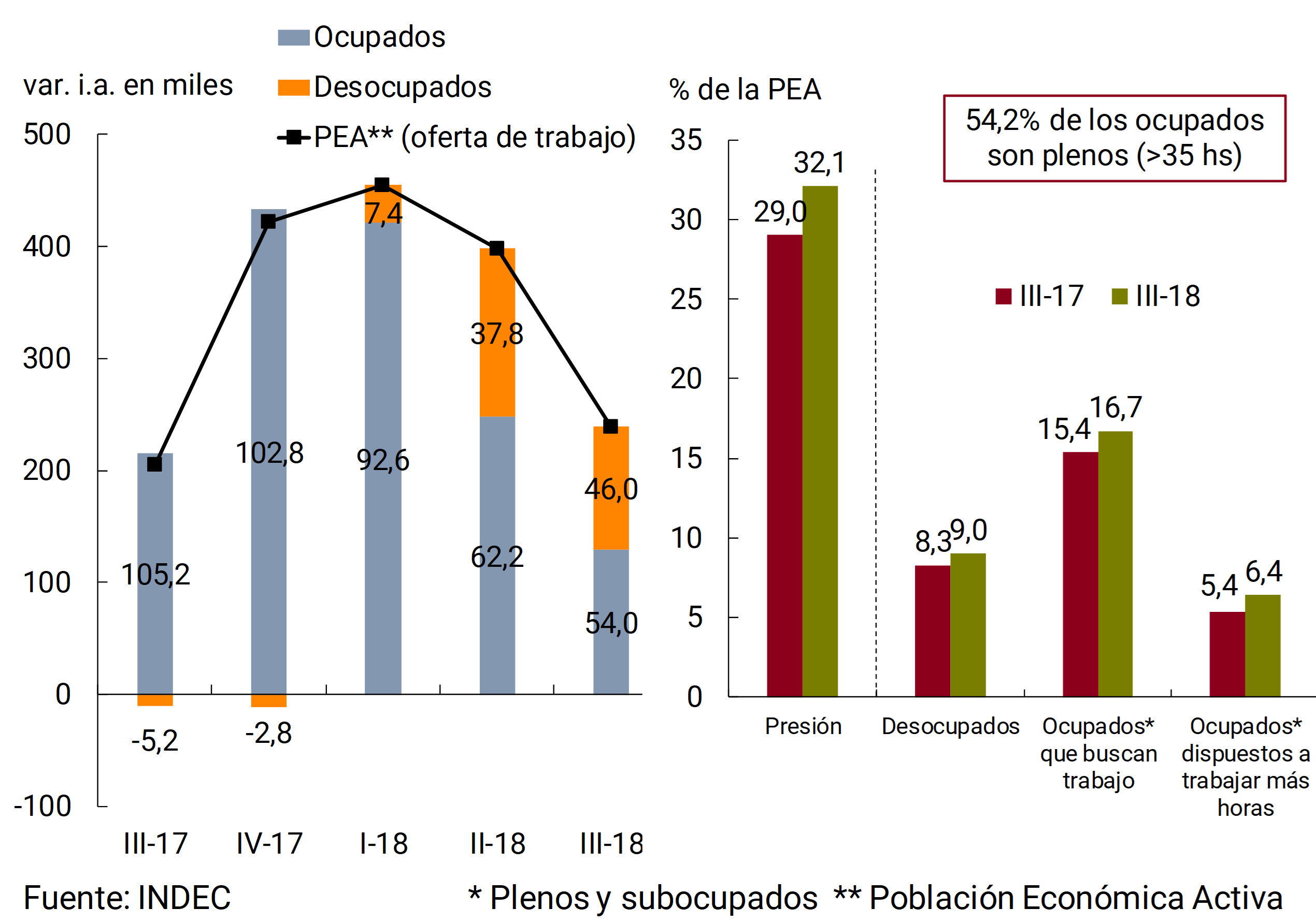
During the third quarter of 2018, the unemployment rate stood at 9%, 0.7 p.p. above the same period of the previous year, according to data from the EPH of INDEC. The increase in the unemployment rate was explained by the rise in the activity rate (+0.4 p.p. y.o.y.) in a context in which the employment rate remained practically unchanged (+0.1 p.p.; see Figure 3.19). In the context described, the pressure of the labor force on the labor market increased. In addition to the increase in job seekers, there was an increase in the number of employed job seekers and non-job seekers who are nevertheless willing to extend their working hours.
Figure 3.19 | Economically active population and pressure on the labour market
In terms of job creation for the coming months, the EIL shows weak hiring prospects. A gradual recovery in employment is expected for 2019 in line with the improvement in activity from the first quarter onwards.
Perspectives
REM analysts expect the economy to bottom out during the first quarter of 2019 and then begin an expansionary phase of the cycle (see Figure 3.20).
Figure 3.20 | GDP Market Projections
Among the factors that would support analysts’ view on the supply side are: the reversal of the decline in the agricultural sector after the drought suffered the previous year and the prospects of a record harvest; the continued expansion of sectors in which deregulation promoted their development since the beginning of 2016 (such as energy, agricultural production, meat, dairy and commercial aviation activity); and the boost from activities that produce tradable goods and services favored by the depreciation of the real exchange rate.
During 2019, external demand is expected to contribute positively to growth (see Section 2, International Context). In particular, the strengthening of the Brazilian economy (growth is estimated at around 2.5% in 2019 compared to 1.3% in 2018) would boost non-agricultural exports. Different estimates indicate that, for each point of growth in Brazil’s GDP, Argentina’s GDP grows between 0.2 p.p. and 0.7 p.p. in the medium term (Adler and Sosa, 2012; De Cárdenas et. al. 2015; Chen 2016, among others)15.
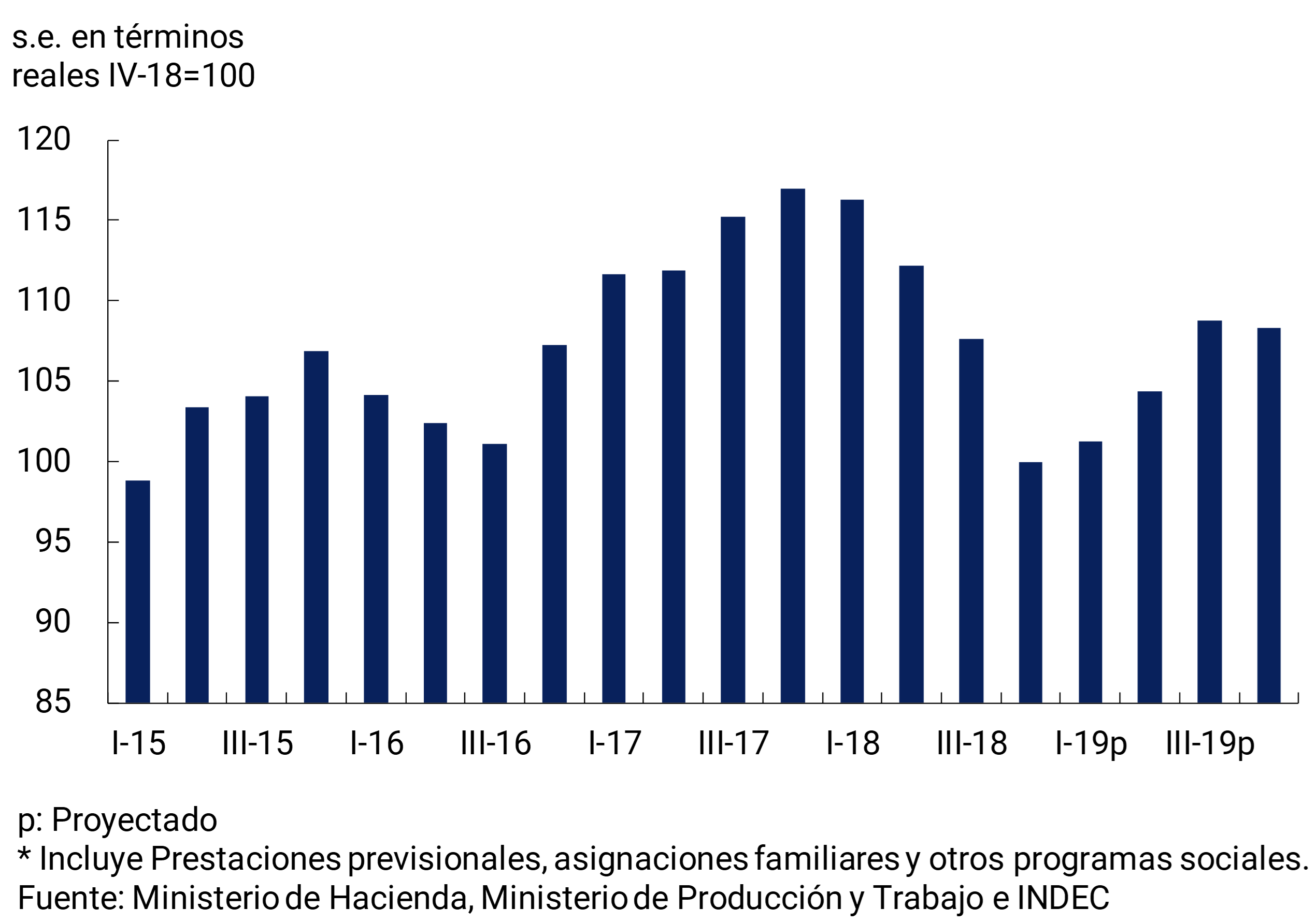
On the side of internal absorption, analysts’ vision of a recovery in GDP during 2019 would imply a gradual revival of private consumption. This expectation would be based on the real recomposition expected in formal wages and social transfers16 (see Figure 3.21). From the gradual improvement in activity, private investment would also begin to regain some dynamism. The gradual recovery of domestic spending will partially reverse the strong compression that imports experienced in the second half of 2018 and that contributed to the economy correcting its current account deficit (measured seasonally adjusted) from -6.6% of GDP in the third quarter to -1.2% in the fourth. In any case, in a context of good prospects for the export sector, the economy is expected to converge in the coming period to a small current account deficit. The expected reduction in the fiscal deficit will also contribute to this result, so that the Argentine economy will have simultaneously eliminated two sources of vulnerability that affected its aggregate performance in the last stage.
Figure 3.21 | Social Transfers of the National Non-Financial Public Sector* (real)
Some risk factors that could condition this scenario of progressive recovery of activity are those that come from the international context, despite the recently observed improvement (See Section 2. International Context). Internally, the upcoming renewal of positions at all levels of government is another risk factor to consider. As is often the case in emerging economies, pre-election cycles can add elements of volatility in domestic financial markets and, through this pathway, affect agents’ spending decisions.
4. Pricing
After the strong acceleration of inflationary records and the potential unanchoring of expectations in September and October, inflation rates for the last two months of 2018 of the year showed a clear decline, although they are still at high levels. The launch of the new monetary scheme, together with a more accelerated convergence to the primary fiscal balance, contributed to stabilizing the financial and exchange rate situation and, through this route, made it possible to begin to recover the nominal anchor for inflation expectations. Despite the decrease in price increases in the last two months of the year, 2018 closed with a cumulative inflation of 47.6%, the highest annual rate since 1991. The sharp rise in annual inflation was associated with a change in the structure of relative prices in favor of tradables (in particular, food), reflecting the real depreciation of the domestic currency. An increase in the relative price of public services (particularly in the Transport category) was also observed, although to a lesser extent than in previous years. Taking into account the lags with which monetary policy operates and the already announced increases in public service rates (mostly concentrated during the first part of 2019), the disinflation process is expected to be gradual. Market analysts’ expectations still anticipate inflation to stand at 28.7% by the end of 2019, although with an appreciable decline in the monthly records expected during the second part of the year.
Figure 4.1 The change in the monetary policy regime led to a reduction in inflation in the latter part of the year
Until the end of the third quarter of 2018, there was a continuous depreciation of the peso that resulted in a systematic rise in inflation. The peak of this process was verified in September/October of last year. The figures for both months were around the highest values since the exit from convertibility, with the exception of April 2002 when inflation rose by 10.4% (see Figure 4.1). The core component of inflation increased again, and averaged 4.5 percent per month in the months of greatest exchange rate stress (peaking at 7.6 percent in September, see Figure 4.2).
Figure 4.1 | Retail Prices
Within core inflation, it was goods – whose variations are more sensitive to exchange rate movements – that reflected the increase to a greater extent. In contrast, private services, of a less tradable nature and whose evolution is more linked to the purchasing power of wages, showed more limited increases in the period.
Figure 4.2 | Core inflation

The launch of the new monetary scheme, together with an acceleration of the fiscal effort in pursuit of primary equilibrium, contributed to reducing pressures on the foreign exchange market, attenuating the main mechanism of recent inflationary impulse. The general price level thus reduced its rate of change to 2.6% monthly in December. Although it was considerably below the values observed in previous months, this inflation rate is still high and is above the records of the end of 2017 and the beginning of 2018.
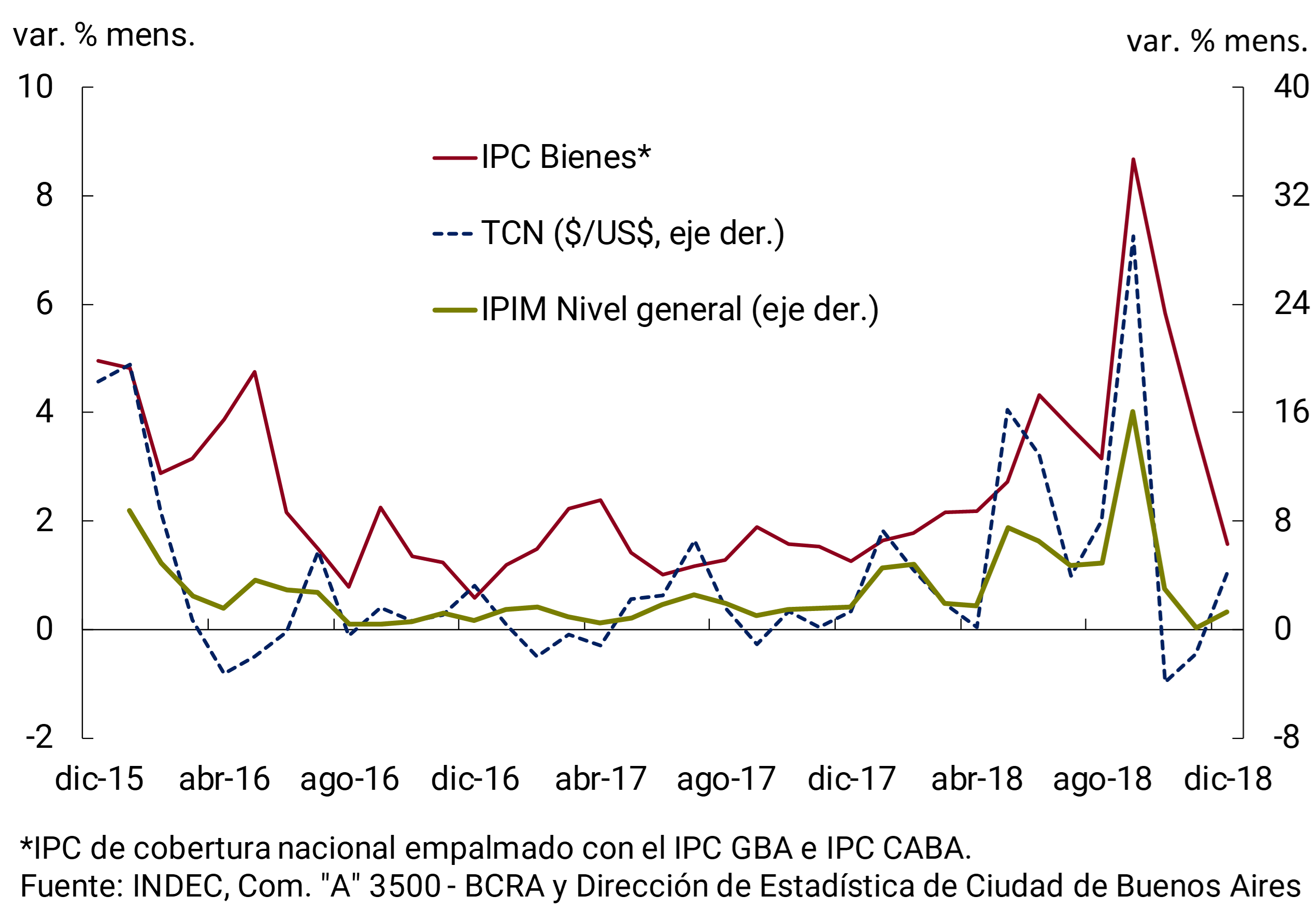
The moderation in the rate of increase in retail prices was mainly explained by the behavior of goods, in a context of lower exchange rate uncertainty. After the 8.7% increase they experienced in September, the prices of goods in the CPI gradually reduced their rate of increase until reaching a monthly rate of 1.9% in December. This behavior was also verified in the wholesale price indices, composed almost entirely of goods, which amplified the dynamics of goods in the CPI (in both directions): after having marked a peak of 16% in September, in November and December the IPIM registered increases of 0.1% and 1.3%, respectively (see Figure 4.3).
Figure 4.3 | CPI Goods, IPIM General Level and Nominal Exchange Rate
In this context, in the last two months of 2018, the prices of private services began to gain some dynamism, which in December averaged increases above those of goods. This evolution may have been associated with a certain recomposition of purchasing power that would have tended to occur at the end of 2018, within the framework of the salary updates and income transfers that occurred in the last part of the year (see Chapter 3 Economic Activity).
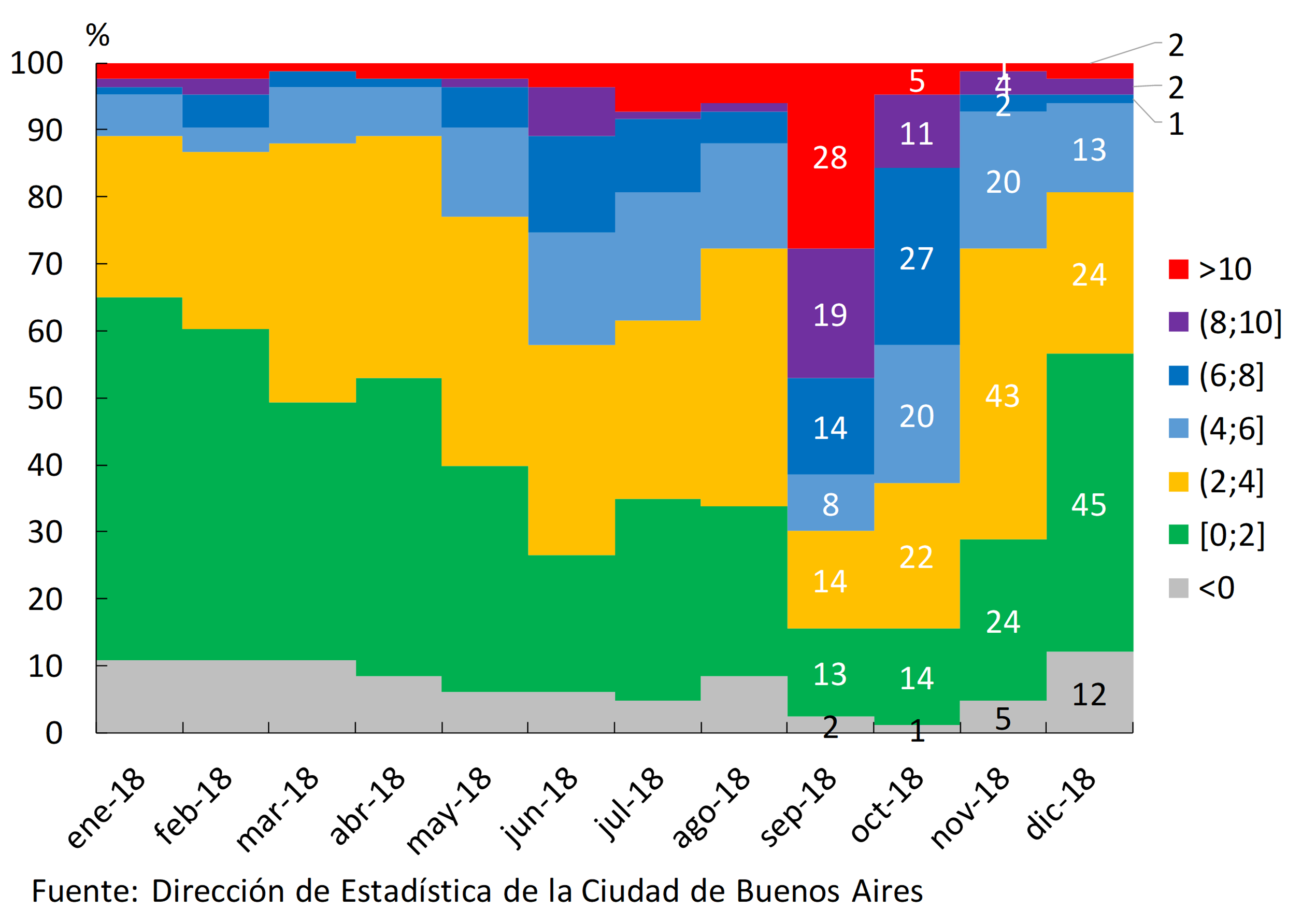
The slowdown in inflation in the last months of the year was accompanied by a reduction in the diffusion of price increases and in their magnitude. Using the classification by purpose of expenditure of the CPI, at the highest level of disaggregation available17, it was observed that, from a minimum in September, the number of CPI classes with positive monthly variations of less than 2% increased from November onwards. The distribution of variations during December was similar to that of the beginning of 2018. Correlatively, the number of classes with monthly increases of more than 10% – which in September had reached 28% of the total – was once again among the lowest levels of the year in December (2.4% of the total; see Figure 4.4).
Figure 4.4 | Distribution of monthly price variations at class level. CPI CABA
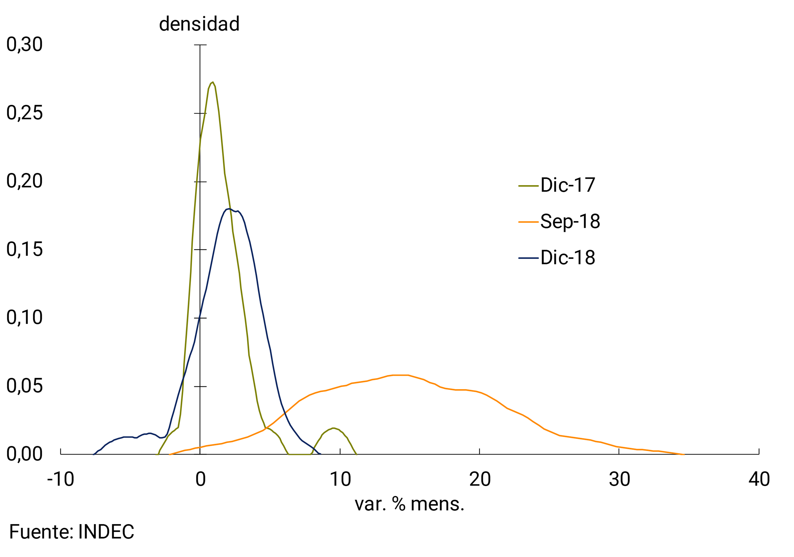
Wholesale indices also registered less widespread increases towards the end of 2018. The distribution of price variations at the IPIM division level was concentrated in December 2018 in values close to 2%, with a decrease in dispersion, after having exhibited a marked increase in the mean and in the dispersion of the distribution in September. However, the distribution has not yet returned to the values of a year ago (see Figure 4.5).
Figure 4.5 | IPIM. Kernel Density Functions
The decline in the inflation rate in the last months of the year was accompanied by a progressive stabilization of inflationary expectations, which had escalated in the context of the inflationary jump of the previous months. Thus, both the median and the average of the inflation forecasts formulated at different terms by REM analysts fell significantly (see Figure 4.6). In particular, the average expected inflation 12 months ahead has been reduced by more than 4 percentage points since the end of August, which enabled the BCRA to eliminate the 60% annual floor in the reference interest rate, complying with the commitment made in September 2018 (see Chapter 5, Monetary Policy).
Figure 4.6 | REM Inflation Expectations

4.2 During 2018 there was a change in relative prices in favour of tradable
productsIn any case, despite the reduction in price increases recorded in the last two months of the year, 2018 closed with a year-on-year variation in retail prices of 47.6%, the highest inflation since 1991. At the sub-index level, the year-on-year growth rate of core inflation was similar to that exhibited by the general level, mainly reflecting the impulses from the exchange rate that were mounted on the previous trend that inflation already had. In particular, food and non-alcoholic beverages were the item with the greatest impact on the rise in the general level. Regulated goods grew above the general level, accumulating a variation of 53.5% YoY. Through their pressure on the cost structure of firms and on household budgets and the consequent wage demands, regulated prices would have thus added second-round effects to the trajectory of core inflation. On the other hand, seasonal goods and services partially offset the dynamics of the general level, with a 35.2% increase in the year (See Figure 4.7).
Figure 4.7 | CPI. Year-on-year changes

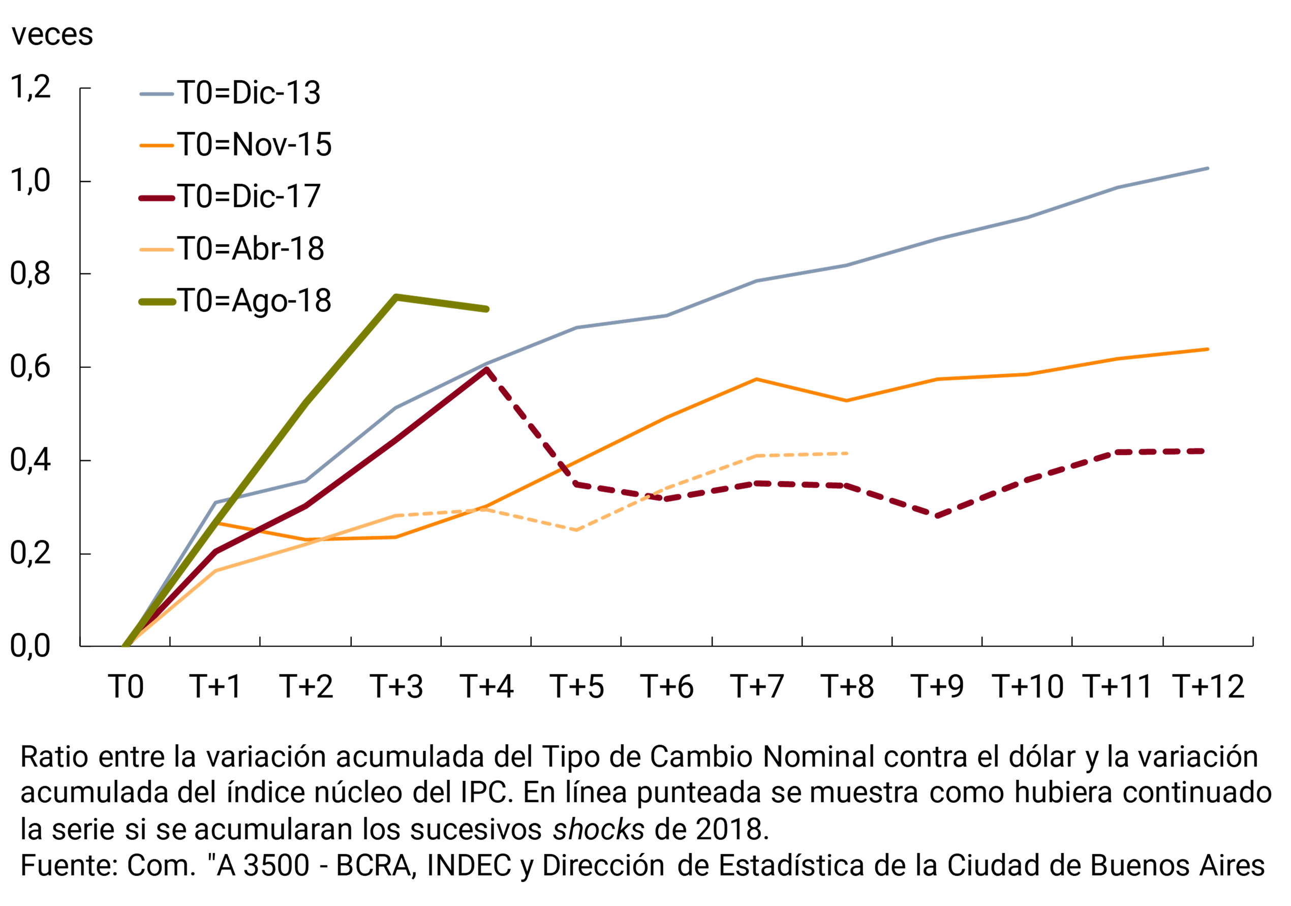
During 2018, the transfer of the rise in the exchange rate (113.2% YoY) to prices (47.6% YoY) was lower than that observed in previous episodes. This lower pass-through (in the order of 40%) allowed a significant correction in the real exchange rate (see Figure 4.8).
Figure 4.8 | Ratio between nominal exchange rate and core inflation
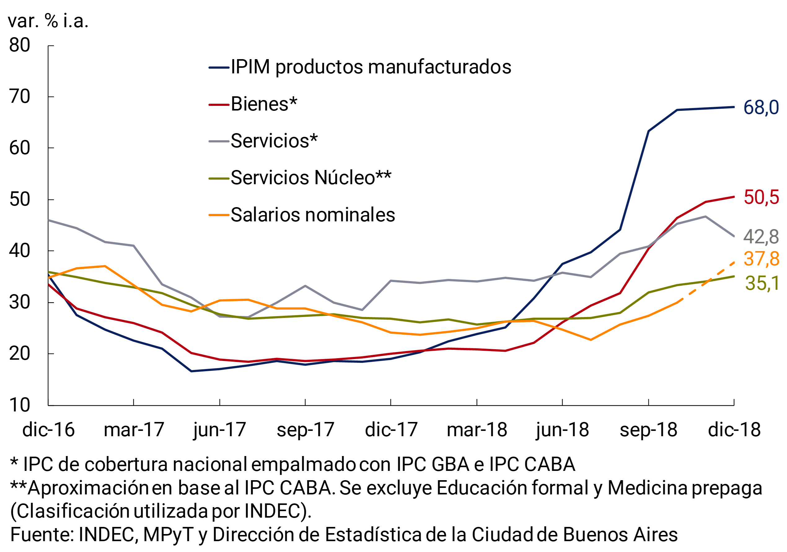
Naturally, it was the “tradable” items that registered the greatest upward momentum from movements in the nominal exchange rate, while the “non-tradable” items (mainly services), and in particular wages, registered more limited variations. In this context of change in the configuration of relative prices, wholesale price indices (with year-on-year increases of between 73.5% and 76.4%), due to their large tradable component, showed a greater sensitivity to the rise in the exchange rate than retail prices (47.6%). Within the wholesale index, the items that reacted the most were imported (105%), followed by the prices of primary products most linked to the price of commodities in international markets (e.g., cereals, oilseeds and crude oil, which exhibited increases of more than 80%), while manufactured products were, within the prices at the factory entrance, those with the lowest accumulated increase (with variations in the order of 70%). Even so, these prices were well above the prices of goods included in the CPI, which have incorporated a greater number of services (distribution, sales force, etc.), which increased by 50.5% YoY last December. Finally, in terms of their largest non-tradable component, there were increases in private services (approximately 35% YoY; see Figure 4.9).
Figure 4.9 | Core Goods and Services, Manufactured IPIMs, and Nominal Wages
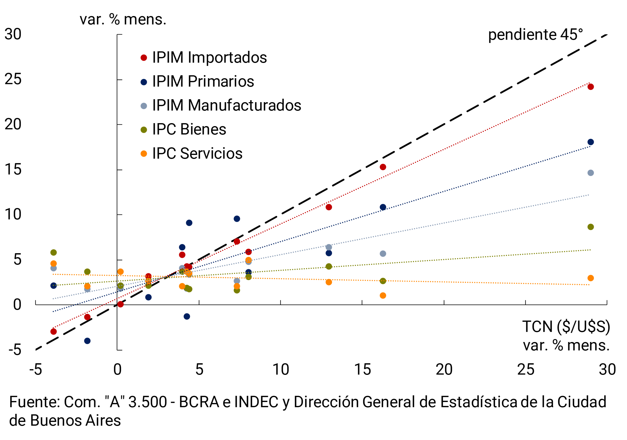
This positive association between the rate of change in the nominal exchange rate and the rate of change in domestic prices according to their different degree of tradability can be clearly seen in Figure 4.10, which shows the intensity of this link for the monthly changes that occurred throughout 2018.
Figure 4.10 | Association between Prices and Nominal Exchange Rate
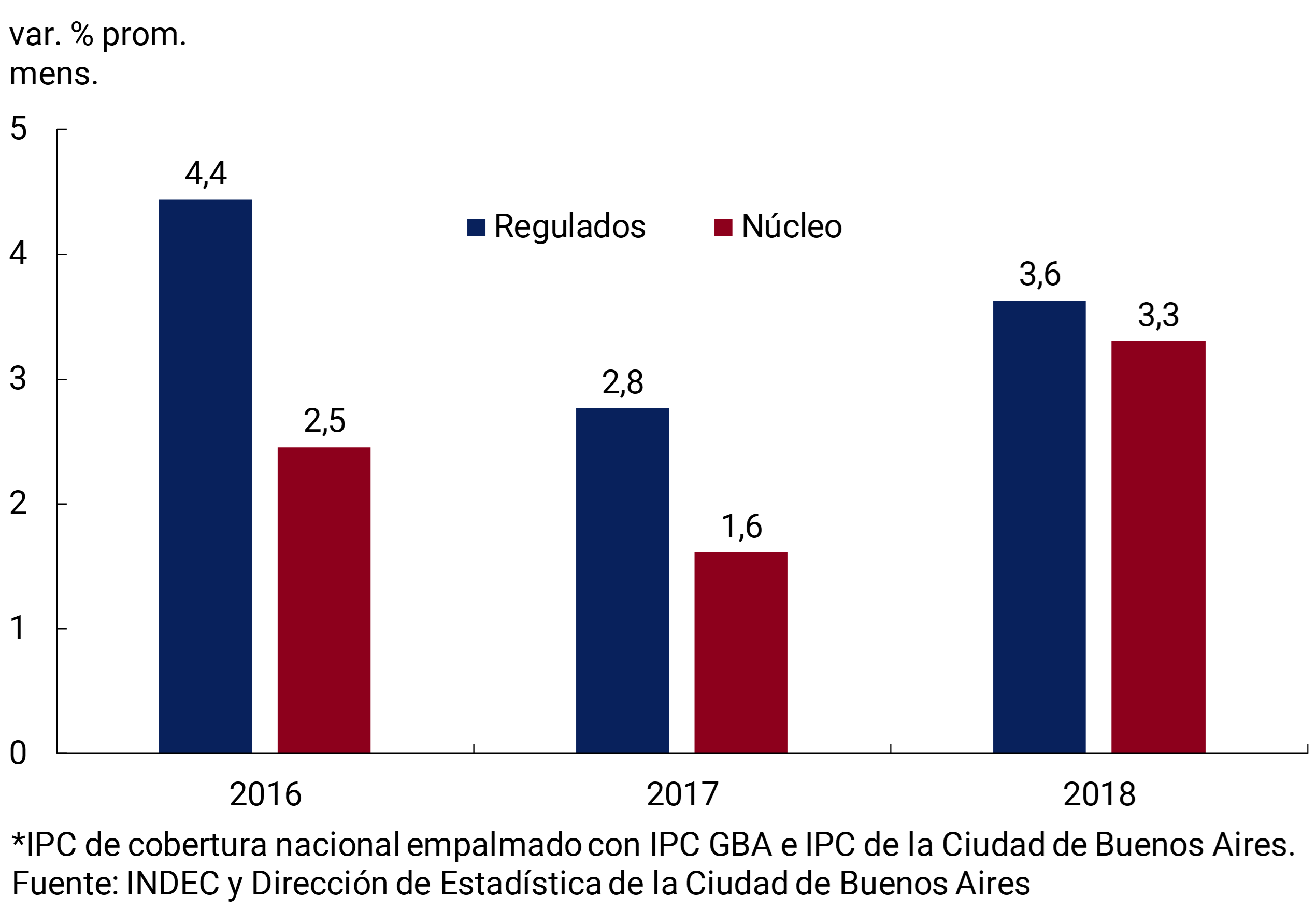
With regard to the recomposition of utility tariffs, although it continued, the change in relative prices in favour of regulated services was considerably lower than that observed in the previous biennium. While in 2016 and 2017 the average monthly rate of increase in regulated goods practically doubled that of core inflation, in 2018 they only exceeded it by 10% (see Figure 4.11).
Figure 4.11 | Core and Regulated CPI*
4.3 Outlook: in the short term, inflation is expected to remain high, due to pending corrections in relative prices, although with a downward trend
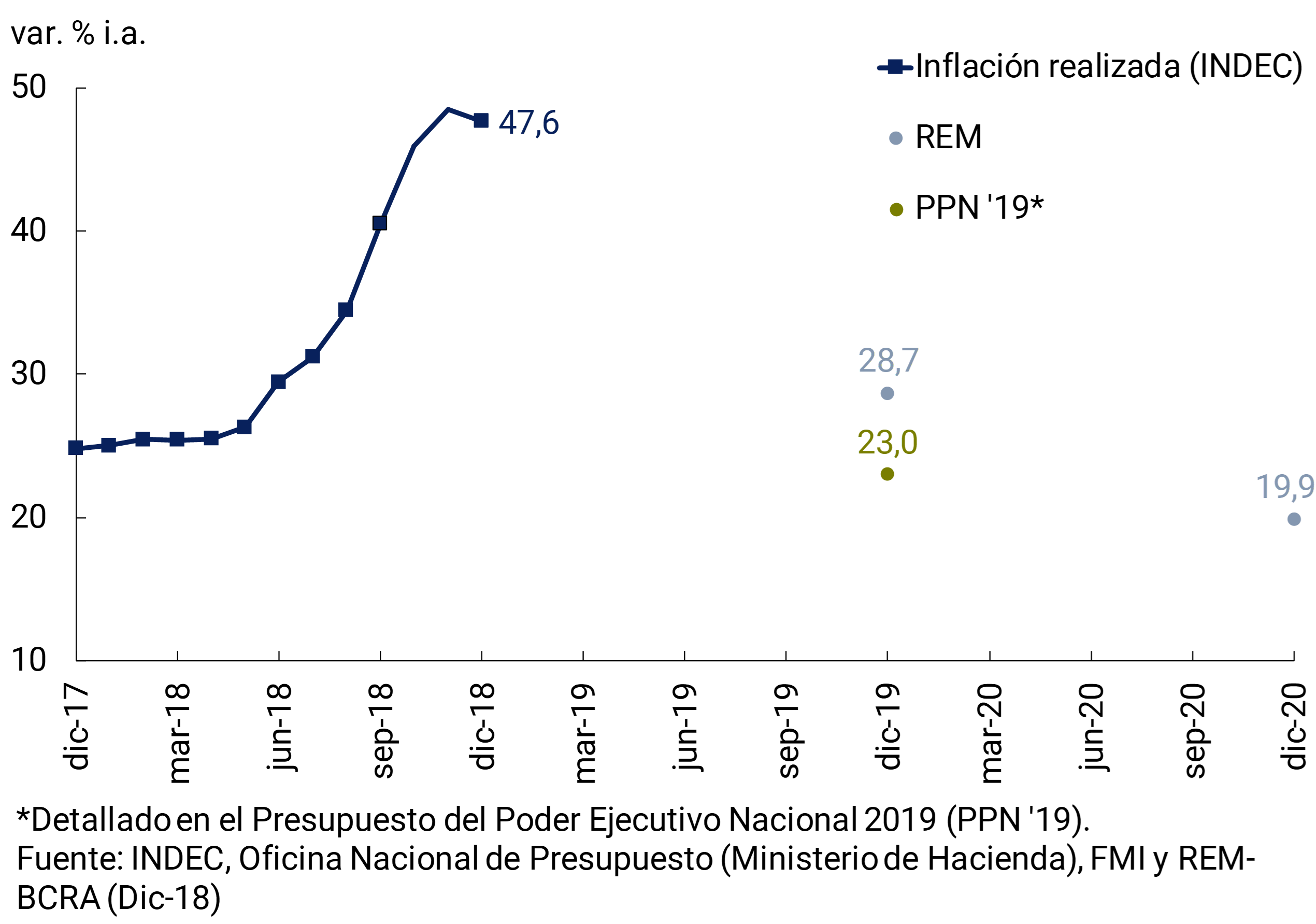
The median of the Market Expectations Survey of Dec-18 anticipates inflation of 28.7% y.o.y. for 2019. This implies a deceleration of 18.9 p.p. compared to 2018. In this sense, market analysts foresee a moderation in inflation lower than that contemplated in the National Budget, which has incorporated 23% y.o.y. for 2019 (see Figure 4.12).
Figure 4.12 | Inflation expectations
For the core component (which covers approximately 70% of the CPI basket) the market anticipates a variation of 26.9% YoY, 1.8 p.p. below the General Level. Given this differential, and assuming that seasonal goods and services (which represent almost 10% of the basket) increase at an identical rate to that of the core component, analysts implicitly expect regulated items to increase 34.4% YoY in 2019.
In addition to reflecting a decrease in expected levels of inflation, market analysts’ forecasts show a much smaller dispersion than in the months of accelerating inflation, showing a reduction in nominal uncertainty. The coefficient of variation of responses declined sharply in the last two months of the year, after peaking in September and October 2018 (see Figure 4.13). Even so, this dispersion of forecasts persists at still high levels, higher than those observed during 2017 and early 2018.
Figure 4.13 | Coefficient of variation CPI General level. Next 12 months

Another source of signal extraction on expected inflation is that which comes from the prices of financial instruments, in particular from the comparison of yields on nominal-rate bonds with those protected from the effects of price increases. Inflation derived from the yield curves of bonds in pesos (LECAPS and Bontes) with respect to that of bonds indexed by CERfrom January 18 to January 7, stood at 26.8% y.o.y. for 2019. This implicit inflation in bond markets also marks a downward path in the year-on-year trajectory of prices and is in line with the projections of REM analysts (see Section 3).
All this seems to reflect that, with the change in the monetary regime, the BCRA began to recover the nominal anchor above expectations and that the forecasts of the financial market and analysts are beginning to align with the guidance provided by monetary policy actions aimed at achieving low and stable inflation.
However, for the first months of 2019, the REM shows a gradual reduction in inflation. The average monthly rate in analysts’ expectations for the first half of the year is 0.4 p.p. above the average monthly rate implied in the second half of the year. The higher figures in the first part of the year would be basically explained by the usual lags with which monetary policy operates and by the existence of certain factors that would put transitory pressures on the evolution of the general price level. On the one hand, public service rates would continue to recover in real terms, with increases concentrated in the first months of the year (see Box. Announcements of increases in utility rates). On the other hand, it is expected that, in a context of progressive recovery in activity levels, there will be some recomposition of some prices that were lagging behind after the exchange rate shock. Along these lines, it is possible to anticipate that, in the first months of 2019, wage negotiations will try to recover part of the loss of purchasing power of 2018 wages, and that this could provide room for a recomposition of compressed retail margins and, in particular, put upward pressure on the prices of private services, whose evolution tended to be more delayed (see Figure 4.14). In any case, it should be clarified that the wage negotiations of each sector will be conditioned by the immediate situation and the prospects of the different branches of economic activity.
Figure 4.14 | CPI ratio goods and IPIM manufactured as a proxy for retail margins

Box. Announcements of utility rate increases
The announcement of increases in public utility rates, concentrated in the first part of 2019, would put a certain floor on the increases in the general price level in the coming months. Recent announcements about updates to gas, electricity, water, and public transportation rates would contribute approximately 4 p.p. to the GBA CPI in that span.
The Ministry of Transportation of the Nation announced the new fare tables for the public transport system of the metropolitan area that imply an increase of approximately 40% for the train and bus. The increases will be applied in a staggered manner between the months of January and March. The tariff tables will come into force in the middle of each month, so the increases will impact the CPI of the first four months of the year. The subway will have an increase of 50.4%, distributed between January and April, adding in January the carryover of the increase from mid-December. In the first month of the year, this is compounded by the drag left by the increase in taxi prices in December. It is worth mentioning that the discounts for social fare (55% discount on the full fare) and for red sube (on package trips) are still in force. Public transport would accumulate a 35% increase in the first four months in the GBA and possibly similar increases will be added in the agglomerations of the interior of the country.
For gas through the residential network, a 35% rate increase was announced in April 2019 at the national level. Electricity service would increase 55.4% in the metropolitan area, with increases of 26% in February, 14% in March and 4% in May and August. The water service in the GBA would have an increase of approximately 49%, impacting in the first two months of the year and starting in May.
With the announced increases, public services (gas, electricity, water and public transport) in the metropolitan area would average a 40% increase during the first half of the year. This increase in public services is similar to that observed between Nov-17 and Jun-18. At the national level (considering the increases in the GBA and gas at the national level) public services would expand at least at a rate of 20% in the first half of the year.
5. Monetary policy
Since October 2018, the Central Bank has implemented a new monetary policy regime based on monetary aggregate targets complemented by the definition of foreign exchange intervention and non-intervention zones. 19 The BCRA committed not to increase the monetary base until June 2019, allowing seasonal adjustments in December 2018 and June 2019, and corrections for non-sterilized interventions in the foreign exchange market.20
In the first months of the new scheme, the Central Bank achieved effective control of monetary aggregates, exceeding the monetary target. Given the dynamics of inflation in that period, this compliance implied a significant reduction in the quantity of money in real terms, which reflects the contractionary bias of monetary policy.
During the last quarter of last year, the exchange rate always operated within the non-intervention zone, although approaching the lower limit of it as the demand for pesos recovered. In January, it was below that limit, which allowed the Central Bank to buy foreign currency in the foreign exchange market by holding daily non-sterilized auctions and thus increase the monetary target.
The contractionary bias of monetary policy made it possible for the Central Bank to begin to regain nominal control of the economy. In this way, the exchange market normalized and inflation expectations began to stabilize. After the strongest impact of the exchange rate depreciation on prices, the inflation rate showed a downward trend, still standing at high levels.
In this context, the nominal reference interest rate (interest rate on Liquidity Bills – LELIQ) registered a downward trend since the October peak, although in real terms it is at high levels. On the other hand, some interest rates in the financial system began to show a downward path following the evolution of the reference interest rate, in a context in which bank credit continued to show a negative trend.
The contractionary bias of the new monetary scheme is expected to be reflected in a reduction in the inflation rate during 2019. However, due to the natural lags in monetary policy and the adjustments of regulated prices and pending wage agreements in the first part of the year, this process will be gradual. At the same time, the economy’s interest rates are expected to continue falling as inflation expectations ease.
5.1 The Central Bank begins to regain nominal control of the economy
5.1.1 Compliance with the monetary target gave a contractionary bias to monetary policy
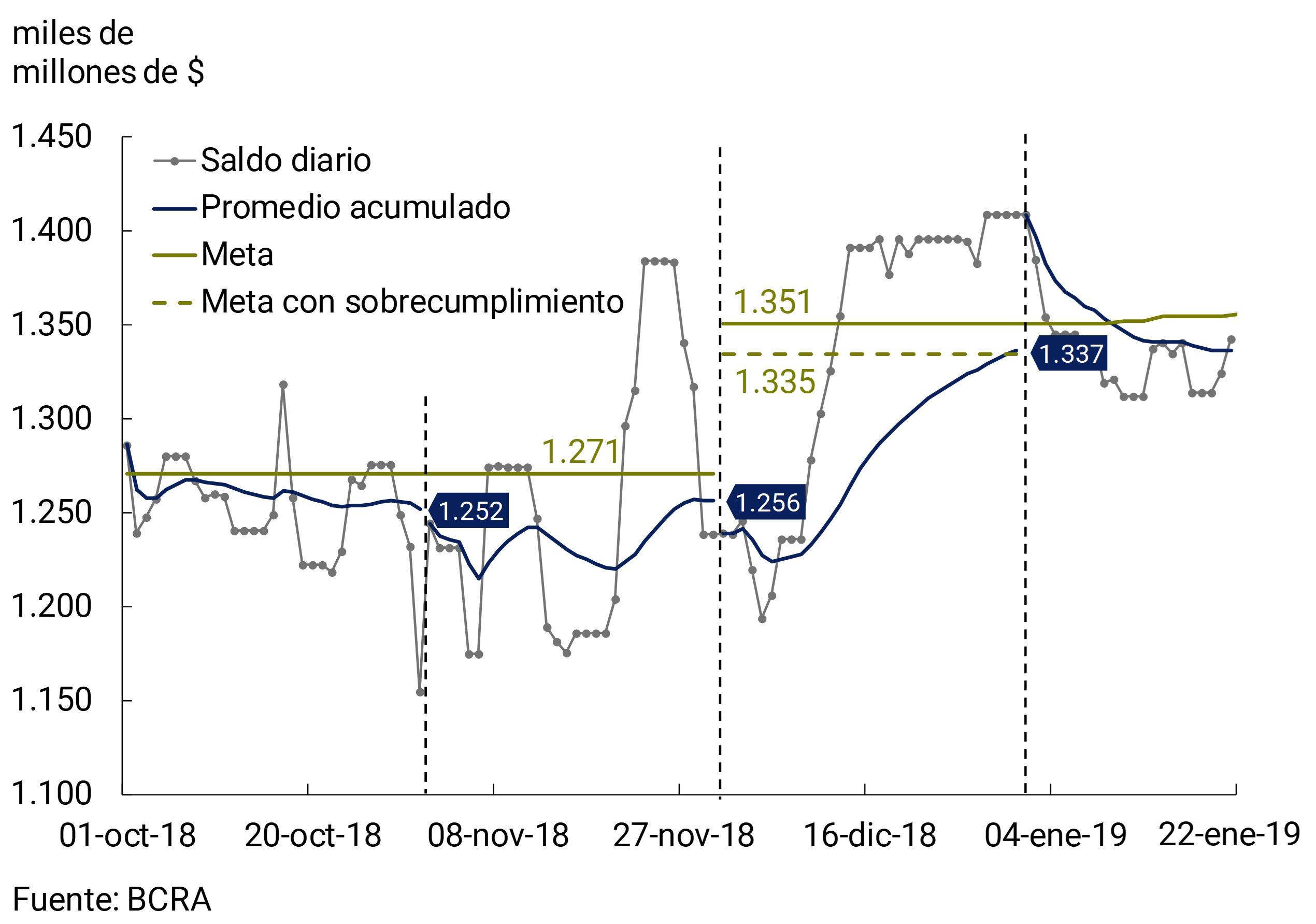
In the first three months of operation of the new monetary scheme, the Central Bank exceeded the monetary base (WB) target by around 1.2%. In order to achieve these goals, the monetary authority held daily auctions of LELIQ, which constitute the main instrument of monetary regulation and can only be acquired by financial institutions. Thus, in October and November, the WB’s monthly averages were $19,000 and $15,000 million lower than the goal of $1,271 billion, respectively. In December, the scheme contemplated an increase in the WB target to $1.351 billion, due to the seasonal growth in the demand for transactional money. The WB’s monthly average in that month was $14,000 million below what was committed (see Figure 5.1). 21
Figure 5.1 | Monitoring the monetary base target
Given the dynamics of inflation in the first months of implementation of the new scheme (see Section 2), meeting the monetary target implied a significant reduction in the quantity of money in real terms, reflecting the contractionary bias of the new monetary scheme. Thus, the World Bank fell 5.1% in real terms and 10.5% in real terms without seasonality between September and December 2018.
In the first twenty-two days of January, the exchange rate was below the lower limit of the non-intervention zone. This allowed the Central Bank to buy foreign currency on several occasions and increase the monetary base with the pesos resulting from these operations, in accordance with the scheme of foreign exchange interventions provided for in the new monetary regime. Thus, the BCRA acquired US$240 million in the foreign exchange market, which was reflected in an increase in the WB’s target for the month of January from a monthly average of $1,351 to $1,356 billion. 22 During the first twenty-two days of January, the cumulative average of the World Bank reached $1.337 billion, $19 billion below the target forecast for the month.
The fulfillment of the monetary commitment has an important pillar in the elimination of transfers from the Central Bank to the Treasury announced in June of last year. Thus, the amount transferred in all of 2018 reached $30,500 million (0.2% of GDP), with a contraction of $39,400 million in the third quarter of the year and with transfers equal to zero thereafter. This factor is reinforced by the Ministry of Finance’s objective of reducing the primary deficit of the public accounts to zero this year.
5.1.2 The foreign exchange market was normalized
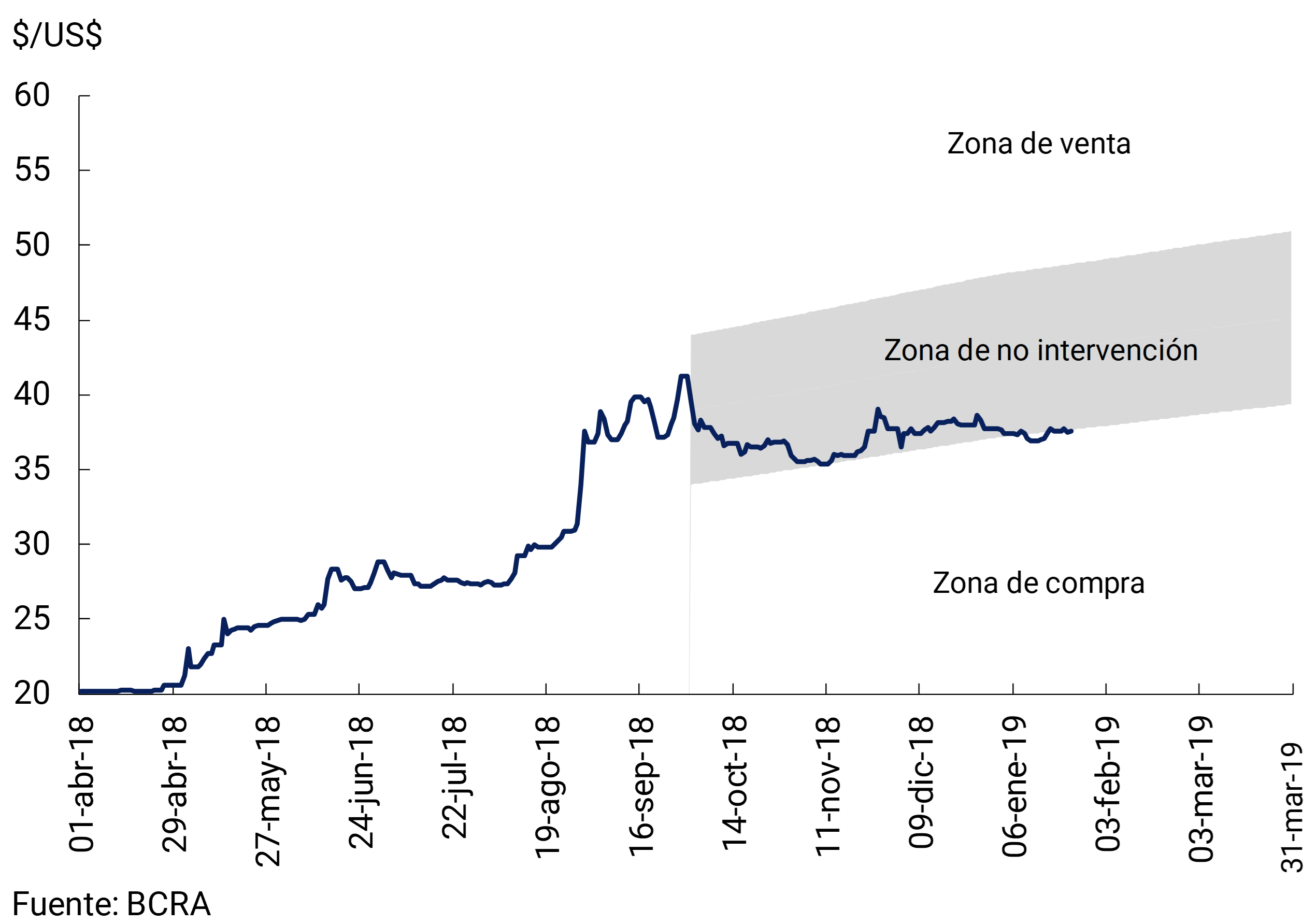
The non-intervention zone was initially between $34 and $44 per dollar, and during the fourth quarter of 2018 it was adjusted daily at a rate of 3% per month. During the first quarter of 2019, the limits of the non-intervention zone are updated daily at a monthly rate of 2% taking as a reference the limits in force as of December 31, 2018 (see Figure 5.2).
The contractionary monetary policy, together with the design of the new exchange rate scheme, contributed to the normalization of the exchange market. Thus, in the last quarter of last year, the exchange rate operated within the non-intervention zone, although approaching its lower limit as the demand for pesos recovered. This FX market dynamic is further highlighted in the face of the international financial uncertainty observed in December 2018 (see Section 1). In January, helped by a more favorable external financial context, the exchange rate was slightly below that limit, which led the monetary authority to buy foreign currency in the foreign exchange market through daily auctions that were not sterilized. Thus, the exchange rate went from $40.9 per dollar at the end of September to $37.6 per dollar on January 22, which implied an 8.1% drop in the U.S. currency (see Figure 5.2). Likewise, the reduction in financial volatility allowed the Central Bank to contract its selling position in dollar futures to zero, which at the end of September 2018 reached US$3,600 million.
Figure 5.2 | Scheme of non-intervention zones and foreign exchange intervention
5.1.3 Inflation expectations stabilize, inflation rate and benchmark interest rate are reduced
The new monetary scheme allowed the Central Bank to begin to regain nominal control of the economy. Thus, twelve-month inflation expectations fell since the implementation of the new regime, 2.9 p.p. for the CPI General Level and 4.1 p.p. for the Core component between the REM measurements of August and December 2018. 23 For its part, the inflation rate began to show a downward trend, after the strongest impact of the exchange rate depreciation on prices, although it remains at high levels (see Section 2). 24
By setting a target for the quantity of money, the benchmark interest rate was determined by the supply and demand for liquidity in LELIQ’s daily auctions, until it reached a level consistent with the commitment to zero growth of the monetary base. After reaching a maximum of 73.5% annually on October 8 as a result of the implementation of the new monetary scheme, the benchmark interest rate began to fall. The fall in inflation expectations for twelve months made it possible to eliminate, on December 5, the “floor” of 60% per year for the interest rate of the LELIQ, to which the Central Bank had committed at the beginning of the new monetary scheme. However, throughout the month, the increase in demand for transactional money above the historical seasonal adjustment interrupted this trend. Thus, the working capital held by the public (the main component of the WB) grew 0.7% in real terms without seasonality in December, after showing a systematic real contraction during the first eleven months of 2018 of the order of 30%. 25 The downward trend was resumed in January of this year, when the benchmark interest rate fell again to 56.9% annually on the 22nd (see Figure 5.3). Despite this fall in the nominal rate, the real interest rate (ex ante) remains at high levels.
Figure 5.3 | LELIQ: Interest rates on LELIQ tenders

5.1.4 Factors underpinning the sustainability of the monetary regime remain
The gradual recovery of nominal control of the economy is taking place without deteriorating the main factors that underpin the sustainability of the monetary scheme, such as the adjustment of external accounts and the dynamics of non-monetary liabilities.
Although the multilateral real exchange rate fell from the peak at the end of September last year, in mid-January it was 30% above the average recorded in the period from mid-2016 to March 2018 (prior to the beginning of the exchange rate turbulence). At the same time, it remains at levels similar to those at the end of 2011, when the economy was in a current account balance close to equilibrium (see Figure 5.4).
Figure 5.4 | Multilateral Real Exchange Rate
The current level of the real exchange rate is contributing to the adjustment of the external accounts, in addition to the impact of lower economic activity on import demand (see Section 3). In fact, since the beginning of October last year, there has been a lower daily demand for foreign currency from net importers and individuals, either for hoarding or tourism, for whom the purchase of foreign currency fell from a daily average of US$160 million in the third quarter of 2018 to US$38 million in the fourth quarter of the same year (-76%) (see Figure 5.5).
Figure 5.5 | Daily net purchases of banknotes in the Foreign Exchange Market (20-day moving average)
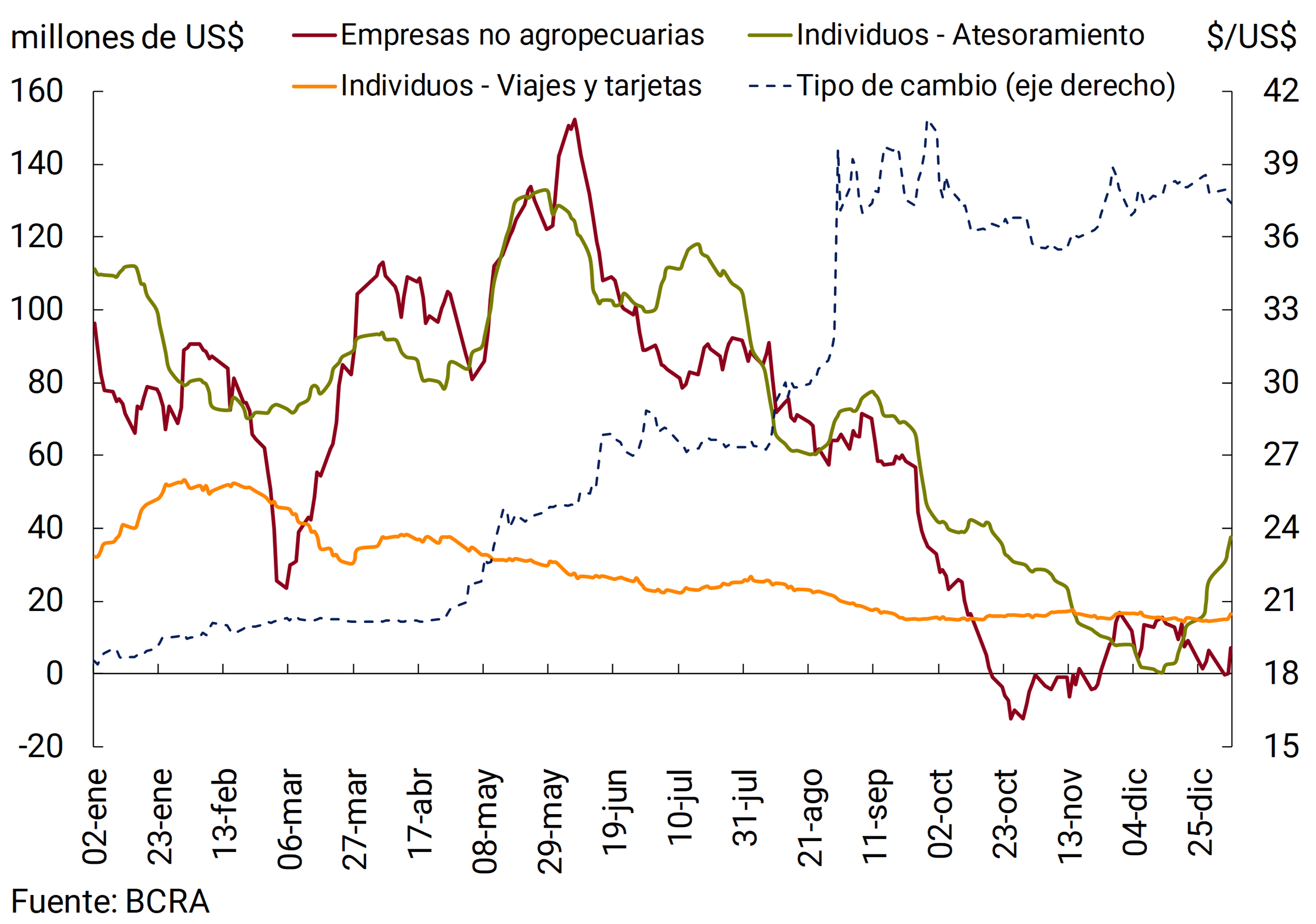
In mid-January 2019, international reserves reached about US$66.4 billion, a level higher than that observed before the beginning of the period of exchange rate turbulence in April last year (see Figure 5.6). Given that in the last quarter of 2018 the exchange rate was not located at any time outside the non-intervention zone, the monetary authority did not carry out purchase and sale operations in the foreign exchange market.26 As of January of this year, the exchange rate was below the lower limit of the non-intervention zone. which allowed the Central Bank to buy US$240 million through daily auctions of foreign currency in the first twenty-two days of the year.
In any case, the main factors that explained the variation in reserves since September last year were mainly the support tranches of the International Monetary Fund in October and December 2018 (2nd tranche: US$5,700 million and 3rd tranche: US$7,600 million), framed in the Stand-by agreement, and the supplementary currency swap agreement with the Bank of the People’s Republic of China for CNY60 billion reached at the beginning of December (equivalent to US$8,800 million).27
Figure 5.6 | BCRA International Reserves

The new monetary scheme implemented by the BCRA implied a reduced expansion of its remunerated liabilities in pesos, so the monetary authority has a reasonable margin to meet its objectives. Although the stock of LELIQ grew from $432,851 million to $836,004 million between September 28, 2018 and January 17, 2019, in December of last year the dismantling of LEBAC was concluded, through which the $340,581 million of these instruments were canceled (see LEBAC disarmament box). As a result, total liabilities remunerated in pesos (LEBAC, LELIQ, net passes and NOCOM) increased only 4% in that period. 28
When the comparison is made against the stock prior to the start of the dismantling of LEBAC in August last year, the fall in remunerated liabilities was 22% in nominal terms. In terms of GDP, the balance of these instruments went from 8.0% in July last year to 5.2% in January of this year, a level similar to that of the beginning of 2016, while in terms of international reserves it went from 0.7 to 0.3 times in the same period (see Figure 5.7).
Figure 5.7 | BCRA’s remunerated liabilities in pesos in terms of GDP and international reserves

It should be noted that, with the total cancellation of the LEBAC, the only holders of instruments issued by the Central Bank became the local financial institutions, which gives greater stability to the demand for these instruments, due to the rules that financial institutions must comply with and that the Central Bank itself dictates in order to preserve the stability of the financial system.
The completion of the dismantling of LEBAC also led to a modification of the reserve policy. At the end of September, the Central Bank had resolved that the minimum cash requirements for the increase in fixed-term deposits could be fully integrated into Liquidity Bills (LELIQ). This measure sought to encourage the capture of fixed terms in pesos and reduce the spread between the reference rate and the rate of fixed-term deposits, in particular, at times when pesos were freed up due to the LEBAC cancellation program. In fact, private fixed-term deposits in pesos grew at a rate of more than 10% per month in October and November, and the spread between the reference rate and the average rate of private fixed-term deposits narrowed by more than 900 basis points between September and December. Given that each institution had its own rate of increase in fixed-term deposits in this period, the proportion of minimum cash requirements that can be integrated by deposits in pesos was different between institutions, even though the term structure of their time deposits was identical. Thus, once the dismantling of LEBAC was concluded, the Central Bank decided to modify the structure of minimum cash requirements with the aim of simplifying the current scheme and transforming the incentive to increase fixed-term deposits since October of that year into a stimulus to extend the terms, calibrating the modification in such a way that it would not impact the level of the monetary base. 29
Box. The LEBAC disarmament process was completed in December 2018
In mid-August of last year, the Central Bank announced a program to cancel LEBAC. These liabilities of the monetary authority had been at the center of the scene in the exchange rate turbulence that began in April. The source of instability in demand for these instruments was that they could be acquired by non-residents (who have very large short-term positions relative to the size of the domestic financial market) and by domestic holders other than banks (who are also sensitive to changes in portfolio decisions).
The stock of LEBAC had been formed as a result of the sterilization of the monetary financing of fiscal deficits and the sterilization of losses from sales of dollar futures contracts prior to December 10, 2015, and the acquisition of international reserves by the monetary authority as of December 10, 2015. reaching around one trillion pesos in July 2018 (8% of GDP).
To implement the cancellation schedule, it was established that in each auction starting in August, the Central Bank would offer LEBAC to non-bank entities for an amount less than the maturity amount, while to banking entities it would only offer NOBAC for 1 year and LELIQ for the total maturity (which can only be acquired by financial institutions). It was also defined that financial institutions could only participate in the primary tenders of LEBAC on behalf of non-bank third parties, and could not sell their remaining LEBACs in the secondary market to non-banking entities. This was complemented by the Ministry of Finance holding auctions of Treasury Bills in pesos on the maturity dates of LEBAC with the aim of generating an attractive investment alternative in pesos and with the modification of the minimum cash requirements for time deposits so that financial institutions would make them more attractive in terms of interest rates.
The disarmament process included five tenders under the detailed modality and ended on December 18. As a result, the LELIQ gained ground, consolidating itself as the Central Bank’s main instrument of intervention, and the total remunerated liabilities in pesos (net passes, LEBAC, LELIQ and NOCOM) fell from $1,078,553 million to $700,998 million between August 14 and December 18 (see Figure 5.8). Thus, a factor that had contributed to last year’s financial turbulence was eliminated, while the stock of interest-bearing liabilities of the Central Bank remained at a level that gives a reasonable margin of maneuver to the new monetary scheme. At the same time, the only holders of instruments issued by the Central Bank became local financial institutions, which gives greater stability to the demand for these instruments.
Figure 5.8 | Evolution of the Central Bank’s interest-bearing liabilities in pesos

5.2 Impact of the new monetary scheme on the financial system
5.2.1 The fall in the reference interest rate was transmitted to money market rates
Interbank market interest rates showed a downward trajectory in line with the reduction in the benchmark interest rate, following the rise generated by the financial turbulence since April last year and by the implementation of the new monetary scheme in early October (see Figure 5.9). Thus, the 1-day call and third-party pass rates fell 12 p.p. and 11 p.p., to reach average levels of 57.0% and 52.4% annually in the first seventeen days of January, respectively.
Figure 5.9 | Money Market Interest Rates

5.2.2 Private sector fixed-term deposits responded to the rise in passive interest rates
In contrast to the fall in the benchmark interest rate observed since mid-October last year, the main passive interest rates of the financial system only fell slightly. This dynamic was explained by the changes in the minimum cash requirements implemented by the BCRA, which encouraged greater collection of time deposits in pesos by financial institutions and had a positive impact on the returns on such deposits. 30 Thus, after the increases recorded in September and October, the TM20 and the BADLAR offered by private banks fell 5 p.p. and 4 p.p., reaching average levels of 48.6% and 46.6% annually in the first seventeen days of January, respectively (see Figure 5.10). 31 For its part, the interest rate on retail fixed-term deposits remained stable at around an average of 42% per year between October and December of last year, then fell 1 p.p. in the first seventeen days of January of this year (see Figure 5.10). As a result of this behavior, a reduction in the average spread of the reference rate with respect to banks’ passive rates of 9 p.p. was observed between the months of October and December. On the other hand, interest rates on fixed-term deposits in UVA cut the 2 p.p. increase recorded in October last year, to return to the average levels of September in December (4.7% annually).
Figure 5.10 | Main Passive Interest Rates of Banks
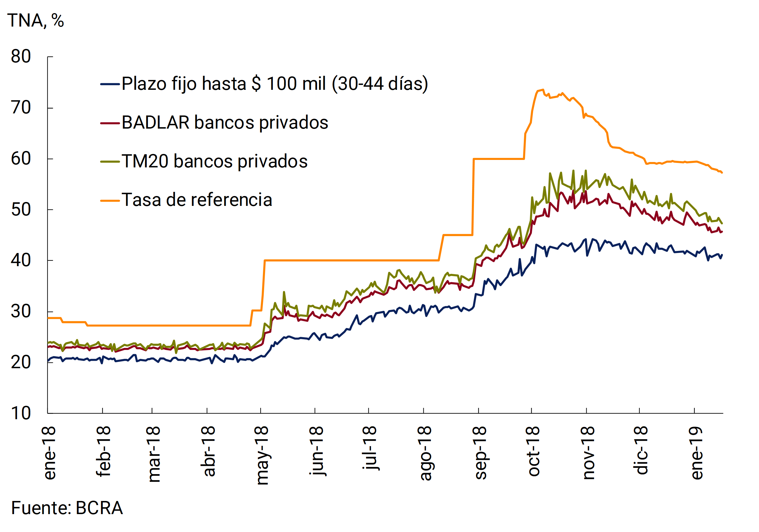
Private sector deposits in pesos exhibited a high dynamism in the fourth quarter of 2018. Thus, they grew at a real seasonally adjusted monthly rate of 1.4%, after three consecutive quarters of contraction (see Figure 5.11). In the year, these placements accumulated a real drop of 4.4%. The increase in the last quarter of 2018 was mainly driven by fixed-term deposits, which increased at a rate of 4.7% per month in real terms without seasonality (+8.7% in real terms in the year), driven by the normalization of the foreign exchange market, the rise in passive interest rates in September and October and the LEBAC cancellation program.
Figure 5.11 | Private sector deposits in pesos (average monthly variation in the quarter – real without seasonality)
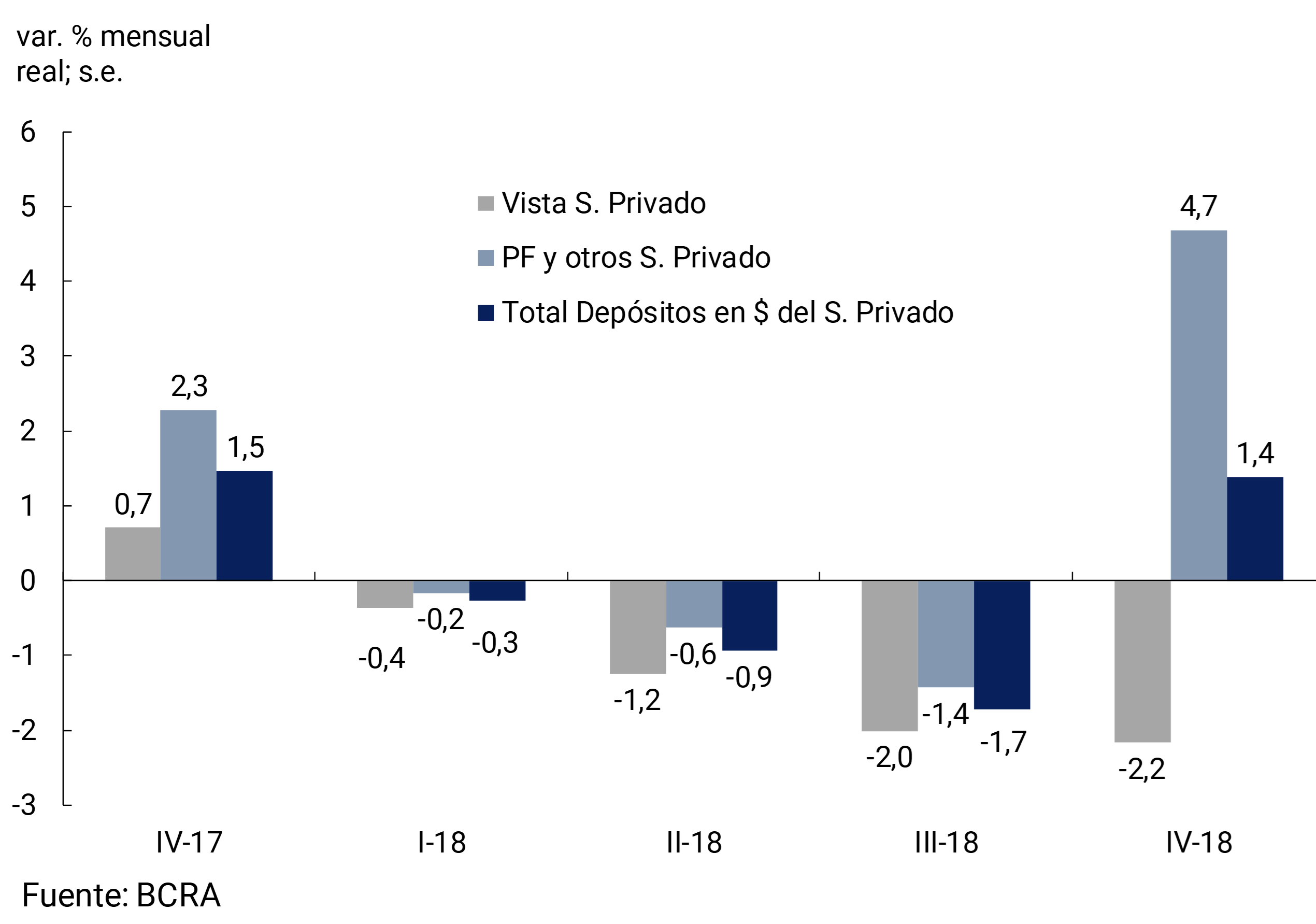
The different agents of the private sector showed disparate behaviors in relation to the evolution of their holdings of fixed-term deposits in pesos during the first eleven months of the year (see Figure 5.12). On the one hand, household deposits showed a relatively stable evolution during the first months of the year, falling 10% in real terms between June and September, at times of greater nominal volatility, and then cutting part of this fall in October and November, in line with the rise in interest rates and the normalization of exchange rate dynamics. For their part, the balances of legal entities grew systematically in the first eleven months of the year, around 40% in real terms, with a marked acceleration as of September as a result of the dismantling of LEBAC and the greater incentives to attract fixed-term deposits based on the measures taken by the BCRA.
Figure 5.12 | Private sector fixed-term deposits in pesos per holder (in real terms)
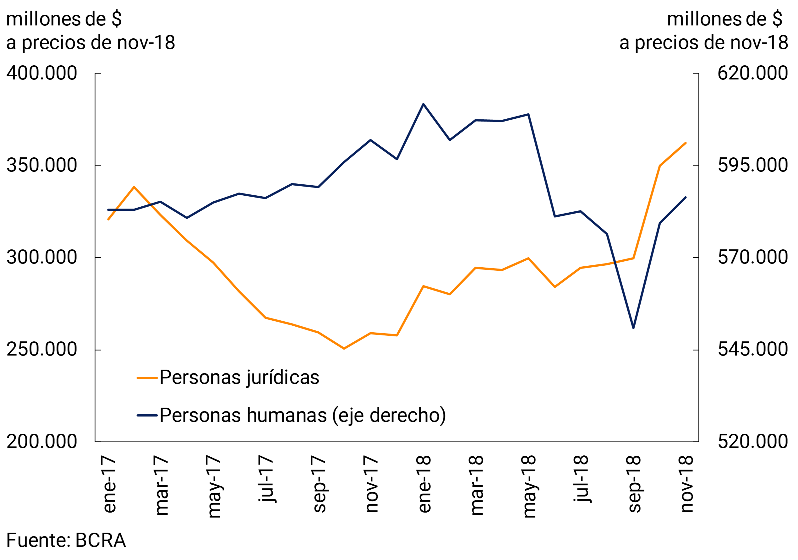
UVA fixed-term deposits in the private sector also reacted to the increase in interest rates, with an average monthly real increase of 16% in the last quarter of 2018, reaching 2.3% of fixed-term placements in December (this share was 0.3% in December 2017). For its part, after the fall in September 2018, private sector dollar deposits grew again in November and December, increasing 1.6% monthly average in the fourth quarter in original currency and reaching a record average stock of US$ 28,503 million in the last month of the year.
With regard to private sector demand deposits, the increase in passive interest rates and the fall in the level of activity drove a non-seasonalized real contraction of their balances of 2.2% monthly average in the quarter (see Figure 5.11). 32 During the year, these placements accumulated a real drop of 16.0%. However, after falling systematically during the first eleven months of 2018, in December demand deposits grew 3.3% in real terms without seasonality, showing a dynamic similar to that evidenced by working capital held by the public (see Section 5.1.3). Thus, the aggregate M2 in pesos of the private sector, which until November last year accumulated a real contraction of 24% in the year, expanded 2.1% in real terms without seasonality in December (see Figure 5.13).
Figure 5.13 | M2 in pesos of the private sector (in real terms without seasonality)
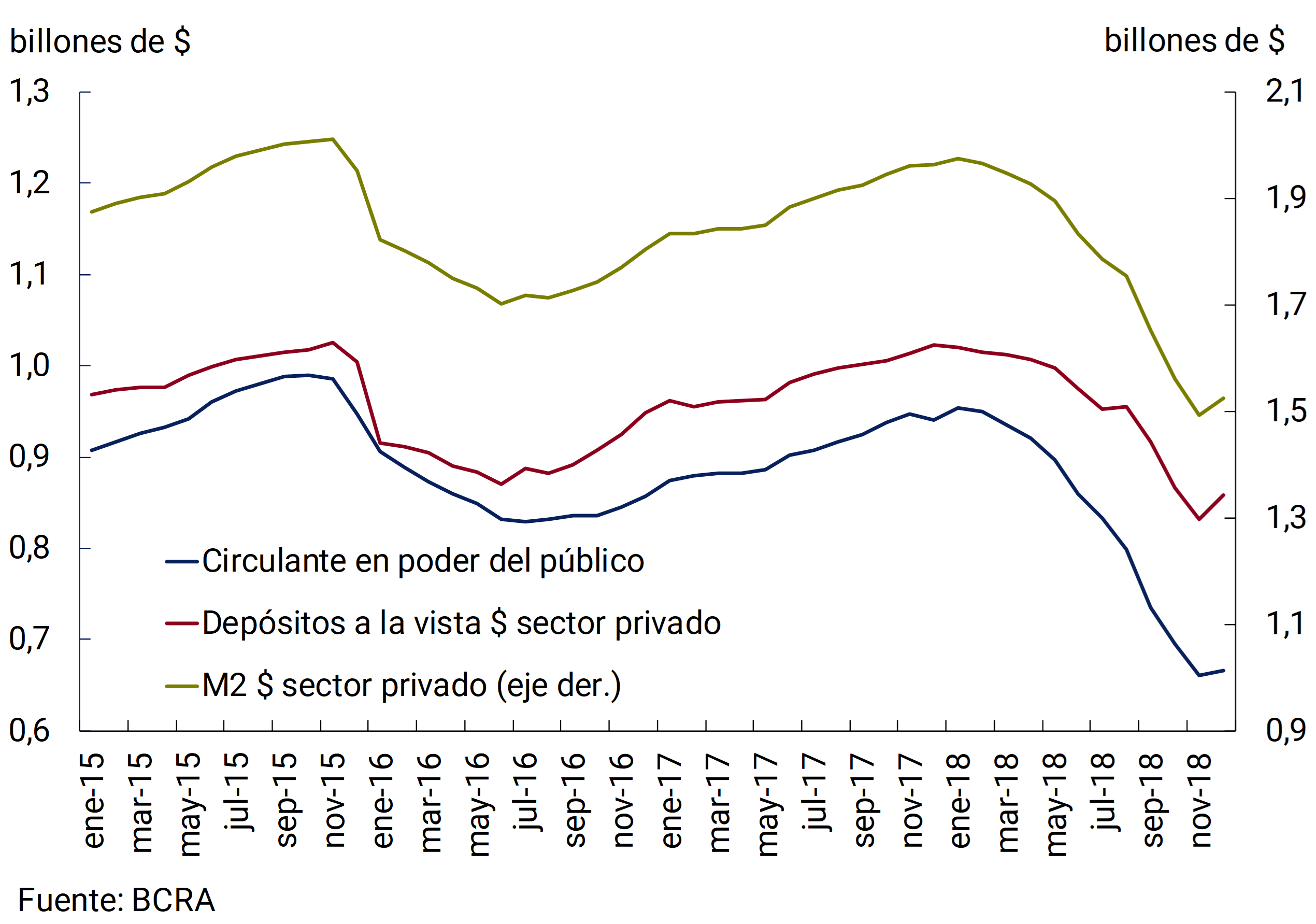
The measures related to the regulation of minimum cash taken by the BCRA in mid-to-late September 2018, which implied increases in regulatory reserve requirements and the application of a marginal reserve requirement on fixed-term deposits, led to ample liquidity in pesos of financial institutions (current account at the BCRA, cash, LELIQ, LEBAC, NOCOM, net passes and 2020 Bond) will continue to grow during the quarter. Thus, it reached 56% in terms of deposits in December, which represented an increase of 9 p.p. compared to September and 16 p.p. compared to the same month in 2017 (see Figure 5.14). 33
The increase in liquidity was mainly explained by the increase in the stock of LELIQ applied to compliance with minimum cash requirements (+13 p.p.), mainly associated with the rise in fixed-term deposits, and by the voluntary holdings of these instruments by banks (+1 p.p.), partially offset by the fall in the LEBAC balance (-4 p.p.) within the framework of the cancellation program initiated in August of the year past.
Figure 5.14 | Liquidity in pesos of financial institutions (as a percentage of deposits)

5.2.3 Bank credit to the private sector maintained the contractionary trend
As of mid-October, some bank financing lines began to show a downward trend in their interest rates, after the increase registered until October of last year. The reduction in interest rates on loans was mainly observed in short-term financing to companies, such as current account advances and document discounting, which showed falls in their average interest rate levels of 16 p.p. and 6 p.p. between October and the first seventeen days of January. respectively (see Figure 5.15). As for the interest rates of the main financing in pesos to households, that of personal loans remained at the maximum levels of October, around an average of 64% annually, while that of credit cards increased 8 p.p. since September, reaching an average of 58.7% annually in December.
Figure 5.15 | Main lending rates of banks

On the other hand, interest rates on the different types of loans denominated in UVA showed disparate behaviors in the last quarter of 2018. While the cost of mortgage and pledge loans remained stable in relation to the average levels of September, around 6% annually and 15% annually, respectively, that of personal loans increased 4 p.p. in the same period, reaching an average of 18.7% annually in the last month of last year.
The combination of higher lending rates and a slowdown in economic activity led to a further contraction of peso-denominated bank loans to the private sector in the last quarter of 2018, which showed an average monthly reduction of 4.9% in real terms without seasonality (see Figure 5.16). In the year, these placements accumulated a decrease of 19.4% in real terms. The reduction was widespread in all credit lines, although those most associated with households fell less than those most demanded by companies. Thus, in the quarter, personal loans and credit cards showed average monthly falls of 2.6% and 1.0% in real terms, respectively, while for advance and document lines they were 6.3% and 5.6%, respectively. On the other hand, mortgage loans and pledges registered average monthly decreases of 1.7% and 3.5% in real terms, respectively. Foreign currency loans to the private sector also contracted in the quarter, at an average monthly rate of 1.4% in original currency (although they accumulated an increase of 4.9% in the year).
Figure 5.16 | Loans to the private sector in pesos (average monthly variation in the quarter – real without seasonality)
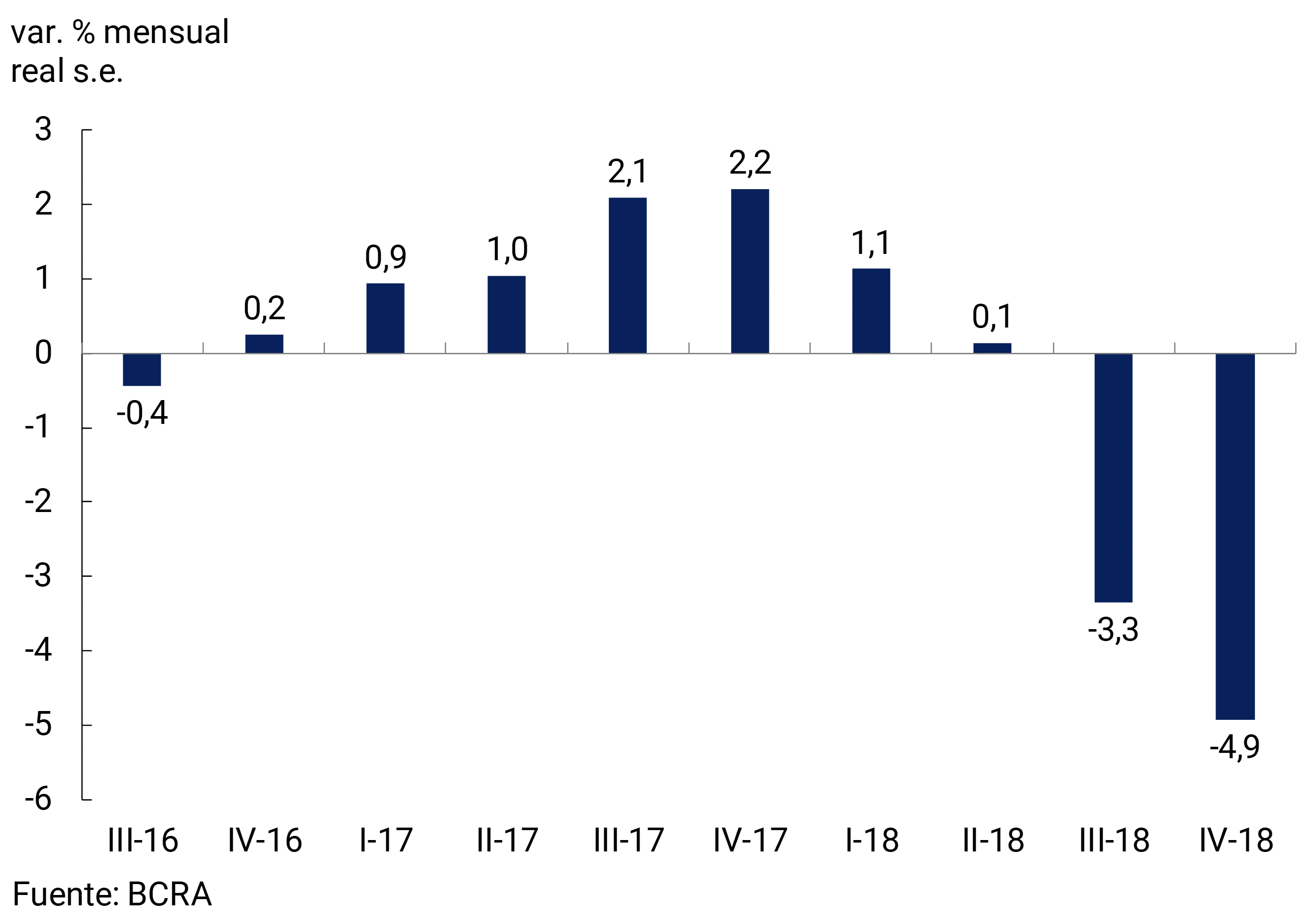
Within the universe of companies, between September and November of last year, bank loans to SMEs showed a smaller contraction than those of the rest of the companies (-13% compared to -16% in real terms, respectively), although in the first eleven months of the year both groups registered a similar real reduction of around 30% (see Figure 5.17). As a result, the share of companies in total bank credit in pesos to the private sector fell from 39% in December 2017 to 33% in November 2018.
Figure 5.17 | Loans in pesos to the private sector per debtor
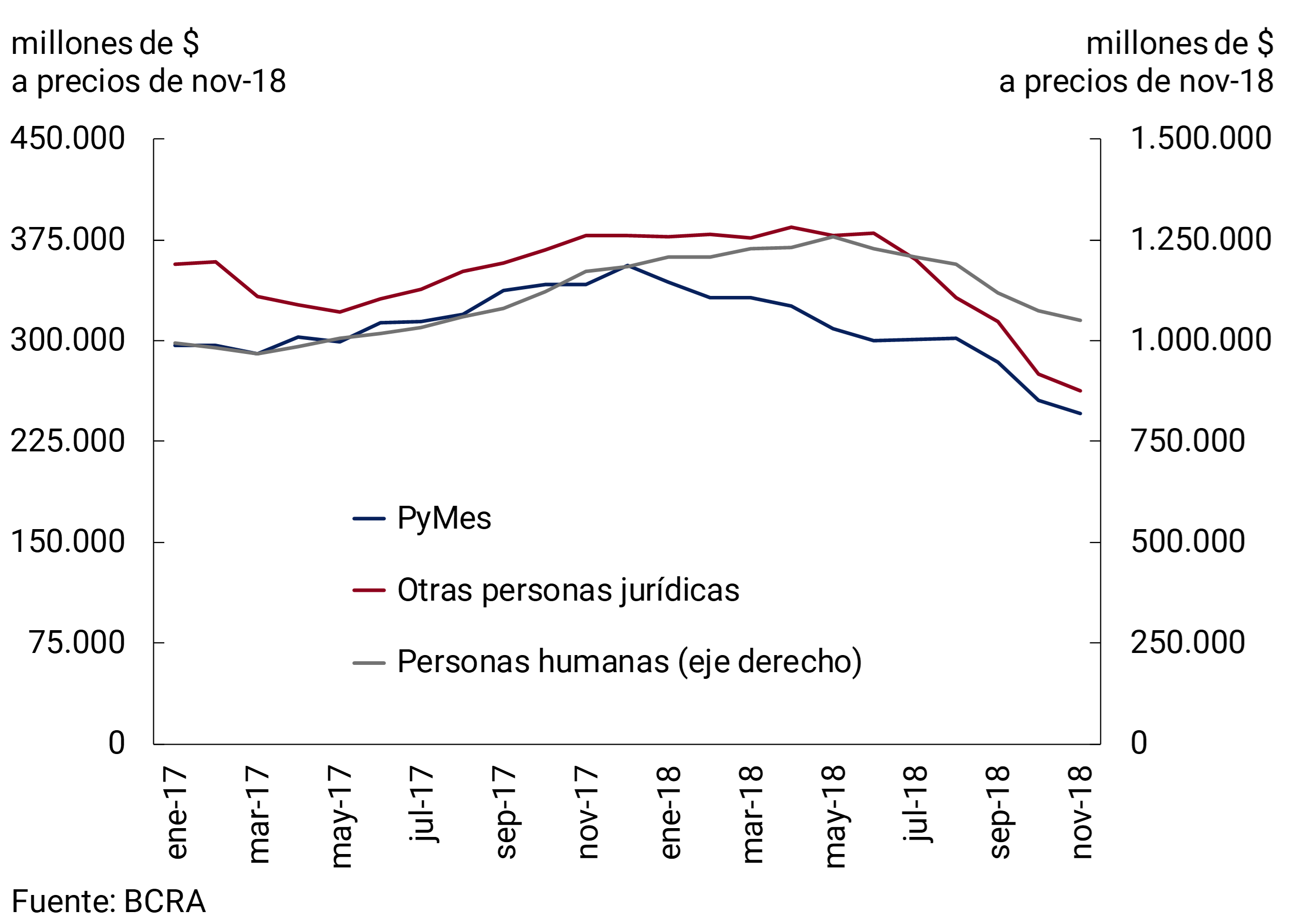
5.3 Outlook
During 2019, the Central Bank will continue to implement the monetary policy scheme based on the control of monetary aggregates, maintaining the objective of zero growth of the monetary base until June 2019 and 1% thereafter until December of the same year, with adjustments in the months of June and December to take into account the seasonal increase in the demand for money (see Figure 5.18). The main tool for controlling the amount of money will continue to be the daily LELIQ auction.
Figure 5.18 | Monetary base targets in 2019
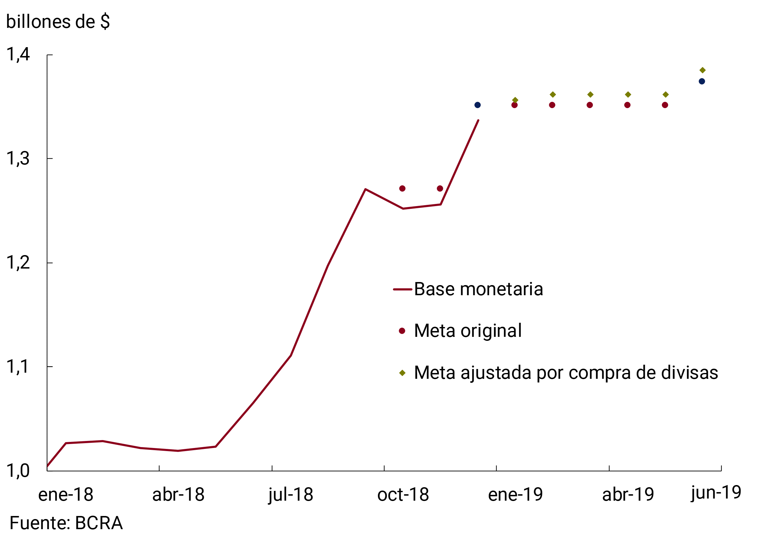
Likewise, the monetary authority will maintain the scheme of foreign exchange intervention and non-intervention zones, as a complement to the monetary base targets. The Monetary Policy Committee defined a daily variation of 2% per month for the limits of the non-intervention zone until March of this year and will establish the pace of updating of the following months in its future decisions.
The contractionary bias of the new monetary scheme is expected to be reflected in a reduction in the inflation rate during 2019. However, a gradual decline in monetary policy is expected, due to natural lags in monetary policy and pending adjustments to regulated prices and wage agreements in the first part of the year (see Section 2).
At the same time, the economy’s interest rates are expected to continue falling as inflation expectations ease. This reduction in the cost of money and the recovery in economic activity that the main market analysts anticipate from the second quarter onwards suggest an increase in the demand for transactional money this year.
This scenario of normalization of the economy could be affected by some risks, mainly linked to a new episode of volatility in global financial conditions or to the usual uncertainty generated by electoral processes. In this context, a series of factors give the Central Bank room for manoeuvre to moderate the impact that the materialisation of these risks could have on the economy, among which the following stand out: the adjustment that the external accounts are showing, the sharp reduction in remunerated liabilities in pesos, the elimination of transfers to the Treasury (in a context of consolidation of the public accounts) and the reduction of the position of Central Bank futures at zero.
The Central Bank will act cautiously, using all the tools available in the new monetary framework to continue to meet its main objective of achieving low and stable inflation.
Section 1 / The yield curve as a predictor of recessions
The slope of a bond market’s yield curve can be used as a predictor of future recessions. In particular, the yield curve of U.S. Treasury bonds is widely used to anticipate recessionary cycles in that country. The idea behind this predictive ability is that long-term interest rates reflect, among other factors, investors’ expectations about future short-term interest rates. In this way, when the curve flattens or inverts, investors would be anticipating a future cheapening of money in the short term, probably due to the fact that they anticipate fewer investment opportunities, less economic activity and a more expansionary bias in monetary policy (Ergungor, 2016).
Beyond the fact that this theory faces some questions, the fact is that of the last six recessions, five were preceded by an inversion of the yield curve, while in the recession of 1990/91, although the curve did not invert, there was an evident flattening. This can be seen in Graph 1 where the yield differential between the 10-year bond and the 3-month bond is shown.
Graph 1 | Yield curve slope and probability of recession in the US

Various econometric studies found empirical evidence that supports this hypothesis. Estrella and Hardouvelis (1991) find that the slope of the yield curve has a greater predictive power than other leading indicators of GDP, while Estrella and Mishkin (1996) conclude that the yield differential between 10-year and 3-month bonds is an important predictor of recessions two to six quarters in advance. However, these authors caution that it is not clear that this predictive power will be maintained in the future, especially if the Federal Reserve begins to look at the yield curve when making its policy decisions.
A decade after these studies, in the face of a new inversion of the yield curve, Haubrich (2006) analyzes whether or not we are on the verge of a new recession. The author reviews the arguments of Alan Greenspan and other detractors of the use of the yield curve as a predictor of recessions: a) we must look at real, not nominal, rates; b) inflation is much lower than in the 90’s, so the inflation premium of long rates is reduced; c) the Fed gained credibility in its fight against inflation, which became less persistent and easy to reduce. While Haubrich admits that the data show a different relationship between yield curve and GDP growth than in the past, he does not fail to mention that the possibility of recession is “not trivial.” Indeed, a year and a half after the publication of the article, the US economy entered a recession when the subprime mortgage market crisis broke out, triggering the global financial crisis.
While the accuracy of this predictor may have been affected by the long time that short-term interest rates remained at zero (Ergungor, 2016), the recent flattening of the yield curve is beginning to generate uncertainty, to the point that the issue was discussed at FOMC meetings. 34 Moreover, the New York Federal Reserve publishes a monthly estimate of the probability of recession for the next 12 months based on the slope of the yield curve35. This reflects the fall in the rate differential between the 10-year bond and the 3-month bond observed during 2018, but especially in the last quarter. The latest data indicates that the probability of having a recession in December 2019 is 21.35%, double what was predicted a year ago (Graph 1).
References:
• Ergungor, O. E., 2016. “Recession Probabilities”. Economic Commentary, Federal Reserve Bank of Cleveland. Available in: https://www.clevelandfed.org/newsroom-and-events/publications/economic-commentary/2016-economic-commentaries/ec-201609-recession-probabilities.aspx
• Estrella, A., Hardouvelis, G. A. (1991). The term structure as a predictor of real economic activity. The Journal of Finance, 46(2), 555-576.
• Estrella, A., Mishkin, F. (1996). The yield curve as a predictor of US recessions. Current Issues in Economics and Finance, Vol. 2, Number 7. Federal Reserve Bank of New York.
• Haubrich, J. G. (2006). Does the yield curve signal recession?. Federal Reserve Bank of Cleveland, 15.
• Johansson, P. Meldrum, A. (2018). Predicting Recession Probabilities Using the Slope of the Yield Curve. FEDS Notes. Board of Governors of the Federal Reserve System. Available in: https://www.federalreserve.gov/econres/notes/feds-notes/predicting-recession-probabilities-using-the-slope-of-the-yield-curve-20180301.htm
Section 2 / Relative Unit Labour Cost (LURCA)
A country’s international competitiveness depends on the quality of its institutions and infrastructure, level of legal certainty, capacity for innovation in products and processes, tax pressure, labor costs and other production costs, to name just a few of the most relevant and recognized factors in the literature.36
On its own, there is no single indicator whose virtues guarantee to make up for the problems that can be observed in the rest of the determining factors. One of the keys to an economy’s competitiveness is to maintain wage cost gaps with competing countries at sustainable levels. This usually depends on the evolution of both comparable wage costs in a common currency37 and levels of labour productivity. This section analyzes the unit labor costs (ULC) of Argentina’s manufacturing sector38 for the last decade and compares them with those published by the Central Bank of Brazil39.
One of the most widely used measures for international competitiveness comparison is ULC in a common currency (dollars) – see box below. Additionally, the relative unit labor cost (ULC) of Argentina and Brazil is the result of calculating the ratio between the ULC series of both countries.
Simplifying, the calculation of the CLUR is based on the following formula:
CLU (Argentina)= (IS/TCN) / (IPI/T)
Where;
IS= Wage Index of the manufacturing sector (Source: Indec and Ministry of Labor)
IPI = Industrial Production Index (Physical Volume Index of the manufacturing sector spliced with the Value Added of the Manufacturing sector, source INDEC)
TCN= It is the exchange rate between the Peso and the USD, understood as so many pesos per unit of foreign currency.
T = This is the index of Employed Industrial Workers (Source: Indec and then Ministry of Production and Labor)
At last; with the singles series of Argentina and Brazil we get:
CLUR= CLU (arg)/ CLU (bra)
Graph 1 | Relative Unit Labor Cost between Argentina and Brazil
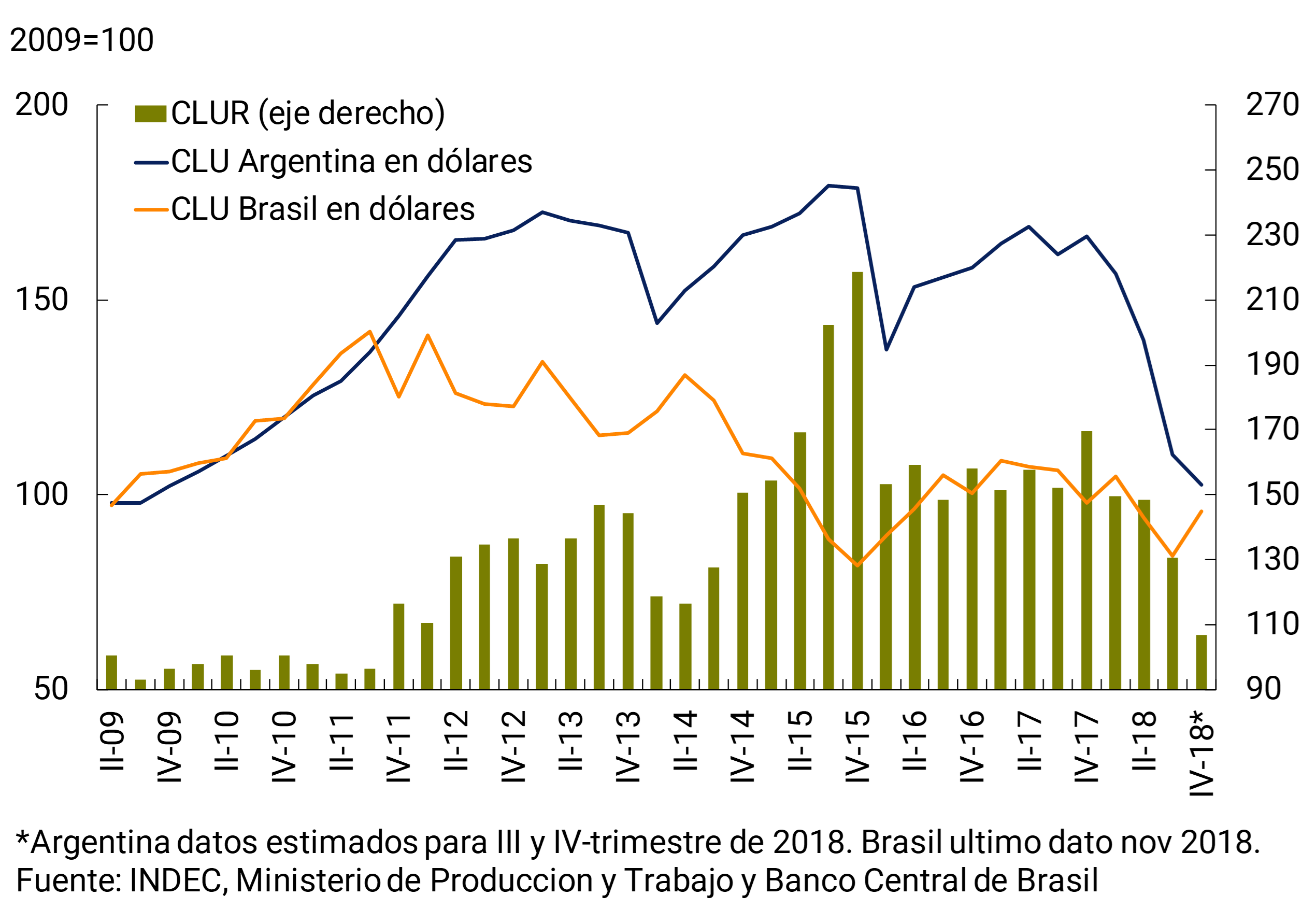
Between 2011 and 2015, there was a progressive widening of the gap in unit labor costs in dollars (CLU USD) in Argentina compared to those in Brazil. This was the result of a growing relative rise in wages in Argentina vis-à-vis those in Brazil, which were not offset by greater relative increases in productivity in our country. From 2015 onwards, although the CLU USD in Argentina showed a slight reduction and those in Brazil showed a slight increase, the cost differential remained at a high level. It was only in 2018, with the strong exchange rate correction of the peso, that the relative labor cost gap between Argentina and Brazil had a significant convergence.
In the medium term, the challenge of raising competitiveness is to deepen reforms that boost labor productivity growth simultaneously with advancing the more comprehensive reform agenda, which include aspects such as improving the quality of its institutions, infrastructure, innovation in products and processes, reducing non-wage labor costs, and improving the quality of its institutions. among others.
Section 3 / Implied inflation expectations in the fixed income market
The prices of financial assets are a source of information to make inferences about the perceptions and expectations of economic agents. In our country, as in other developing economies, public securities are generally the most liquid within the universe of listed instruments. Under this premise, in this section the fixed income market is used to analyze the recent evolution of inflation expectations in Argentina.
In order to obtain the daily evolution of an indicator of inflation expectations 12 months ahead, we begin by calculating daily zero-coupon curves for securities in pesos and securities adjustable by CER. To calculate the zero-coupon curves for a given day, the available prices of the securities considered40 are used, and specific points of the curve are obtained by means of the bootstrapping method. Subsequently, to complete the curve for all the maturities, the Nelson-Siegel 41-Svensson42 model is adjusted from the points previously obtained. This procedure is carried out for each day in the period from 1 January 2018 to 7 January 2019. As a result, two zero-coupon curves (the one corresponding to securities in pesos and securities in pesos adjustable by CER) are obtained for each day.
Once the zero-coupon curves have been calculated, the inflation expectations indicator is computed as the difference between the 12-month zero-coupon rate of the curve of securities in pesos (nominal rate) and that of securities adjustable by CER (real rate).
Graph 1 shows the results obtained. The dotted blue line represents the daily expectations indicator. The solid dark blue and light lines show the 5-day and 20-day moving averages respectively. Finally, the green dots indicate the median of the 12-month inflation expectations surveyed by the REM. The orange segments around each point correspond to the 10th and 90th percentile, and are incorporated as a measure of dispersion in the formation of expectations.
Several elements deserve to be highlighted. First, in general terms, the daily frequency indicator obtained from the term structure of interest rates is well adjusted to the expectations surveyed in the REM. Second, the period in which the discrepancy between the expectations indicator and the median of the REM survey is greater, coincides with an increase in the measure of uncertainty associated with the formation of expectations – noting the average amplitude of the 10th and 90th percentiles between August and November 2018. Finally, over the last two months, both measures of expectations have shown a convergent dynamic.
However, the evolution of the expectations indicator for the period can be better analyzed if it is complemented with the information in Chart 2, which shows the 20-day moving average of the disaggregated indicator as the difference between the nominal rate of securities in pesos not adjustable by CER and the real rate that results from adjustable securities.
The evolution of the series represented in Graph 2 allows us to clearly identify three stages. The first, which runs from the end of April 2018 to the end of August, is marked by the first episode of exchange rate stress, and is characterized by the gradual unanchoring of inflation expectations (twelve months ahead), which went from around 20% to 30%. At this stage, the increase in inflation expectations took place at the same time that the nominal and real yield curves were jointly upwards, reflecting the trend towards the substitution of assets denominated in local currency by assets denominated in dollars. The second stage takes place during the month of September, and has its origin in the exchange rate stress at the end of August. This episode was reflected in a new increase in inflation expectations, which stood at around 40% towards the end of September. With respect to the evolution of nominal and real rates, on this occasion there was evidence of a substitution towards adjustable securities by CER, which put downward pressure on the real rate, which was decoupled from the evolution of the nominal rate. This behavior was reinforced by the contractionary bias of monetary policy, which raised the return on short-term peso assets. The adoption of the new monetary regime marks the beginning of the third stage. In this period, there is a downward trend in inflation expectations implicit in the fixed income market, which from December onwards were back at the previous level, around 30%. In terms of nominal and real rates, the behavior of the last period is consistent with a greater demand for assets in pesos, not adjustable by CER43.
Graph 1 | Indicator of expected inflation 12 months ahead
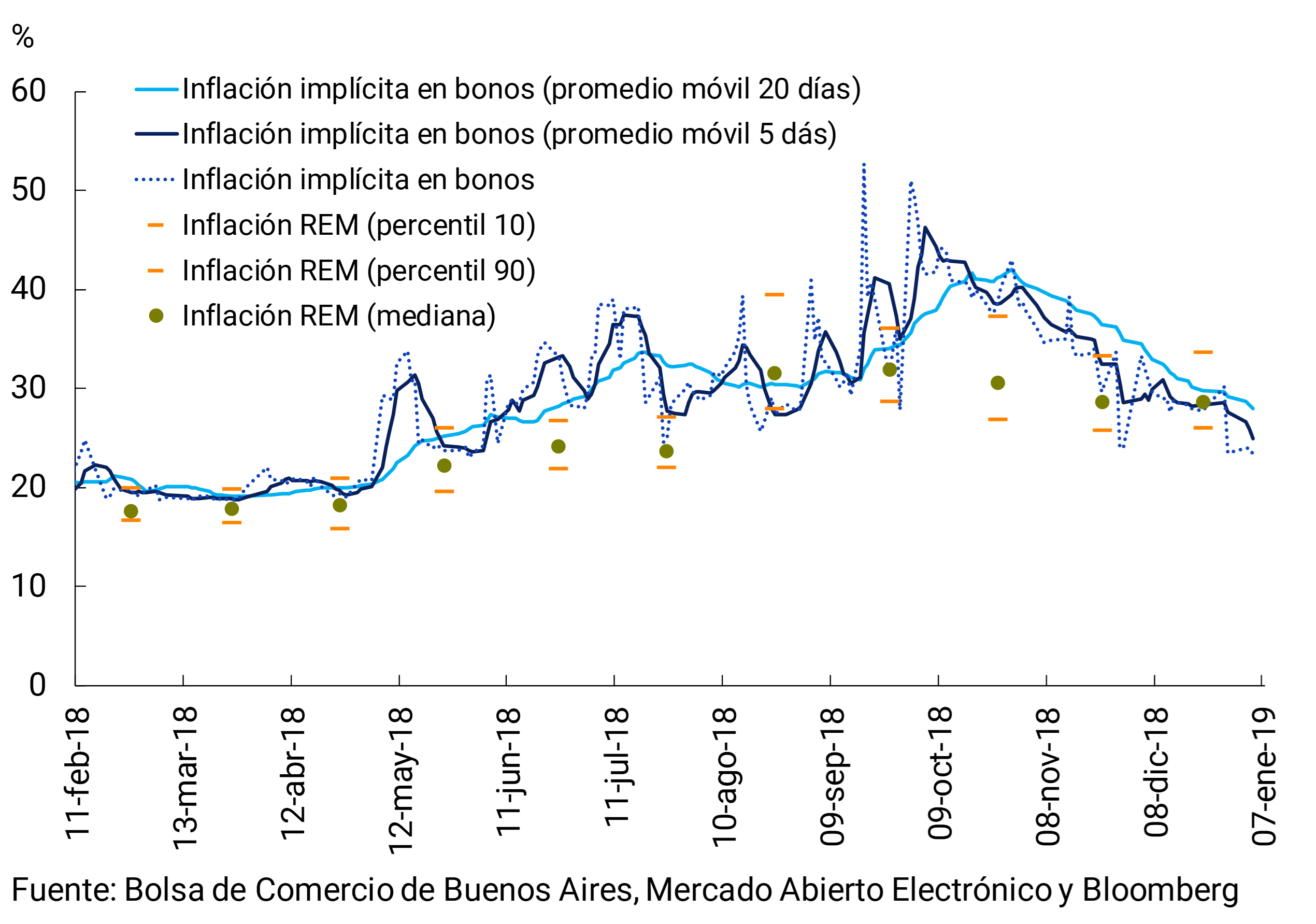
Graph 2 | Decomposition of the expected inflation indicator 12 months ahead
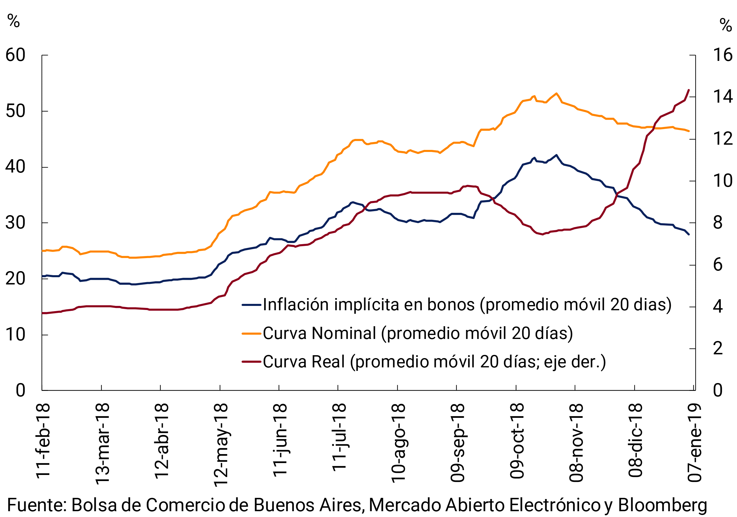
References
1 For more details on what WLTPs are, see this link.
2 The preliminary estimate of German GDP for 2018 released in mid-January shows that GDP would have grown 1.5% in the year, the lowest value since 2013.
3 In October 2017 the ECB reduced its asset purchase programme from €60 billion per month to €30 billion, and from September to December 2018 to €15 billion per month.
4 The Target on the Federal Funds Rate.
5 In the first days of January, progress would be made in the trade negotiations between the United States and China.
6 In the World Economic Outlook of October 2018, the IMF performs in Scenario Box 1. Global Trade Tensions (page 33) an analysis of the possible global impact of these measures. The Box concludes that there would be a loss of global GDP of 0.4% in the long term, in the most adverse scenario of all, if it were to occur.
7 It should be noted that exports of goods were affected by the effects of the drought mainly in the second and third quarters of 2018.
8 Monthly frequency index that includes traditional and non-traditional indicators of the consumption of goods and services. For more details see Section 1/ Private consumption, a variable difficult to follow in real time, IPOM July 2017.
9 The agreement between the National Government and the International Monetary Fund contemplated the possibility of increasing social protection programs focused on vulnerable groups in the face of adverse economic conditions. The adjuster that operated in 2018 was $14,000 million on the primary result target of the National Non-Financial Public Sector on a cash basis. That amount included the extraordinary granting of the one-time sums per child of $1,200 in October and $1,500 in December 2018, after the $400 granted in March 2018. For 2019, the maximum amount of this adjuster amounts to $37,000 million.
10 Decree 1043/2018.
11 Consumer Confidence Index of the Torcuato Di Tella University.
12 The quarterly variations of the IBIF-BCRA indicator are a weighted average of the seasonally adjusted quarterly variations of the ISAC (INDEC), imports of capital goods (INDEC) and national production of capital goods (FIEL). The weights correspond to the weight of construction, investment in imported durable production equipment (EDP) and national EDP in the IBIF of the previous quarter. Between October and November, the ISAC fell 7.4% s.e. compared to the second quarter, imports of capital goods decreased 18.1% s.e. while the national production of capital goods fell 3.3% s.e.
13 The Gross Value Added of the Transport and Communications sector contracted 0.4% s.e. in the third quarter of 2018, slowing down the decline compared to the -3.3% evidenced in the second quarter.
14 In particular, the soybean harvest is expected to reach at least the level of the 2016/2017 season (54 million tons), which means an increase of approximately 44% y.o.y., mainly explained by better yields. On the other hand, corn production for this campaign could register an all-time record (about 53 million tons) growing in this scenario by 24% y.o.y., driven both by higher yields and by a larger planted area.
15 See IPOM of January 2017.
16 Pension benefits and family allowances fell in real terms in the second half of 2018 – due to the acceleration of inflation and the regulatory mechanism that indexes these concepts with a certain lag. In a scenario of a slowdown in inflation during 2019, this mechanism allows us to foresee a recomposition in real terms of these social transfers.
17 This information is only available for the IPCBA and the level of disaggregation used is that of class (level 3). The classification of expenditures adopted by the City of Buenos Aires is the Classification of Individual Consumption according to Purpose (CCIF) and according to this criterion the goods and services that make up the CPI were grouped into 12 Divisions, 37 Groups, 83 Classes, 145 subclasses, 285 sets of products and 628 products.
18 The estimate of implied inflation for 12 months is based on the comparison of the curves of zero coupon rates in nominal pesos and zero coupon rates in real pesos. The first is estimated from the secondary market quotations of the LECAP and the bonds in nominal pesos (Bontes); in the case of the real zero-coupon rate curve, the secondary market quotations of bonds in pesos with CER adjustment are used.
19 For more details on the monetary scheme implemented as of January 1st. of October, see the Monetary Policy Report of October 2018.
20 The monetary base is composed of monetary circulation (banknotes and coins held by the public and held by banks) plus the current accounts in pesos of financial institutions at the BCRA.
21 This level of over-compliance was marginally lower than the $16 billion over-compliance target that had been determined by the Monetary Policy Committee of the Central Bank of the Argentine Republic (COPOM) at its meeting on December 5, 2018.
22 For the month of January, the COPOM defined a limit of US$ 50 million for daily purchases of foreign currency with a ceiling on the increase of the monetary base of up to 2% of the original target.
23 Corresponds to the median of inflation expectations surveyed in the REM.
24 The REM (Market Expectations Survey) is the survey of expectations on the main economic variables that the BCRA conducts with the main local consulting firms and research centers, financial institutions in Argentina and foreign analysts.
25 The other component of the monetary base is the bank reserves, which include the working capital held by financial institutions and their current account deposits in pesos with the BCRA.
26 At the end of December last year, the Central Bank made a direct purchase of foreign currency from the Treasury for US$1,133 million.
27 This agreement complements the bilateral currency swap agreement signed in July 2017. The total amount of swaps, including both agreements, amounts to CNY130 billion (US$19.1 billion).
28 NOCOMs are the Cash Clearing Notes that financial institutions can acquire with their surplus banknotes. They are instruments with a 30-day term that accrue an interest rate equivalent to 1/5 of the reference interest rate. For more details see COM. “A” 6575 and COM. “B” 11760.
29 The new minimum cash requirements will become effective as of January 1st. of February of this year for the largest financial institutions (Group “A”) or linked to global groups of systemic importance, and as of February 1st. of January 2019 for the rest of the entities. For more details on the amendments to the minimum cash policy, see the December 20 (http://www.bcra.gob.ar/Noticias/BCRA-regimen-de-efectivo-base-monetaria.asp) press release and COM. “A” 6616.
30 Effective between 1st. and on December 31, 2018, the BCRA allowed financial institutions to integrate with LELIQ or NOBAC the reserve requirements for the new fixed terms in pesos that they received.
31 The BADLAR rate corresponds to deposits of more than $1 million arranged with a term of 30-35 days, while the TM20 corresponds to deposits of more than $20 million with a term of 30-35 days.
32 Demand deposits include current account deposits and savings bank deposits.
33 During 2018, the minimum cash requirements on deposits in pesos of the largest financial institutions (those that had deposits from the non-financial private sector in pesos at the end of July 2018 for an amount greater than or equal to 1% of the total of these deposits in the financial system) increased by 21 percentage points. In the case of demand deposits, the integration was distributed 5 p.p. with BOTE 2020, 8 p.p. with pesos and 8 p.p. with LELIQ, while in the case of fixed-term deposits it was 5 p.p. with BOTE 2020, 3 p.p. with pesos and 13 p.p. with LELIQ. To this was added, as of September 30, a minimum cash requirement on the increase in fixed-term deposits to be fully integrable with LELIQ and/or NOBAC. Finally, towards the end of December, the structure of minimum cash requirements was modified with the aim of simplifying the current scheme and transforming the incentive to increase fixed-term deposits since October of that year into a stimulus to extend the terms, calibrating the modification in such a way that it would not impact the level of the monetary base. For further details see COM. “A” 6526, 6532, 6550, 6556, 6569, 6575 and 6616.
34 https://www.federalreserve.gov/monetarypolicy/files/fomcminutes20171213.pdf.
35 https://www.newyorkfed.org/research/capital_markets/ycfaq.html.
36 (https://ideasdepeso.com/2017/08/30/el-desafio-de-incrementar-la-productividad-laboral-en-argentina/).
37 Such a comparison of wage costs must necessarily be made in common currency (USD) since what matters for a producer of tradable goods (whether it exports or competes with imports) is its wage costs compared with those of other similar countries, adjusted for labour productivity. This will be relevant for their possibilities of insertion in foreign markets, or to compete in the domestic market with similar products that arrive from other countries of the world.
38 Due to the availability of data, the manufacturing sector is usually used, although it would also be interesting to carry out this analysis for the agricultural, services, commercial, etc. sectors. Notwithstanding the above, the manufacturing sector represents 17% of Argentina’s GDP and 33% of exports are manufactures of industrial origin, additionally 18% of the employees of the formal private sector correspond to industry, which is why it is revealing to analyze this sector in Argentina.
39 https://www.bcb.gov.br/en#!/home.
40 Securities in non-adjustable weights: Letes, Bonte: TO21, TO23, TO26. Securities in New York law or foreign dollars: AA19, AA21, A2E2, AA26, A2E7. Titles that adjust for CER: TC20, TC21, PR13 and DICP.
41 Nelson, Charles R Siegel, Andrew F, 1987. “Parsimonious Modeling of Yield Curves,” The Journal of Business, University of Chicago Press, vol. 60(4), pages 473-489, October.
42 Svensson, L.E.O., 1994. “Estimating and Interpreting Foreward Interest Rates: Sweden 1992-1994,” Papers 579, Stockholm – International Economic Studies.
43 In the last stage, the trajectory of the real rate is dominated by the behavior of the short section of the curve of pesos that adjust for CER. The increase would be less marked if the yield of an instrument with greater liquidity were considered, such as the Discount in pesos (DICP).
Glossary of abbreviations and acronyms
€: Euro
Acum.: Cumulative
AFCP: Portland Cement Manufacturers Association
AFIP: Federal Administration of Public Revenues
AUH: Universal Child Allowance for Social Protection
BADLAR: Buenos Aires Deposits of Large Amount Rate (interest rate paid for fixed-term deposits of more than one million pesos in the 30 to 35-day bracket by the average of banking entities)
BCB: Central Bank of Brazil
BCBA: Buenos Aires Stock Exchange
ECB: European Central Bank
BCRA: Central Bank of the Argentine Republic
BONAR: Argentine Nation Bond
CABA: Autonomous City of Buenos Aires
CEMBI+: Corporate Emerging Market Bond Index Plus
CEMBI+AR: Corporate Emerging Market Bond Index Plus Argentina
ECLAC: Economic Commission for Latin America and the Caribbean
CER: Reference Stabilization Coefficient
FIGURE: Research and Training Center of the Argentine Republic – Central de Trabajadores de la Argentina (CTA)
COICOP: Classification of Individual Consumption According to Purpose
CNV: National Securities Commission
Contrib.: Contribution
S Fuels Energy
DJVE: Affidavits of Foreign Sales
e: Dear
EDP: Durable Production Equipment
EIL: Survey of Labor Indicators
EMAE: Monthly Estimator of Economic Activity
EMBI+: Emerging Markets Bond Index Plus
EMBI+AR: Emerging Markets Bond Index Plus Argentina
EMBIG: Emerging Market Bond Index Global
ENGHo: National Survey of Household Expenditure and Income
EPH: Permanent Household Survey
excl.: Excluding
Fed: Federal Reserve of the United States
FIEL: Latin American Economic Research Foundation
IMF: International Monetary Fund
IMF WEO: World Economic Outlook
FOB: Free on Board (purchase and sale operations carried out by boat)
FOMC: Federal Open Market Committee
GBA: Greater Buenos Aires
A.I.: Year-on-year
IAMC: Argentine Institute of Capital Markets
IBIF: Gross Domestic Fixed Investment
ICC: Consumer Confidence Index prepared by the Torcuato Di Tella University
ICC-INDEC: Construction Cost Index
IGA-OJF: Orlando J. Ferreres General Activity Index
ILA: Leading Activity Index
ILCO: BCRA’s Leading Indicator of Private Consumption
INDEC: National Institute of Statistics and Censuses
INML: Liniers Market Steer Index
CPI: Consumer Price Index of national coverage released by INDEC
IPCBA: Consumer Price Index of the City of Buenos Aires
CPI Cordoba: Consumer Price Index for the Province of Cordoba
CPI GBA: Consumer Price Index of Greater Buenos Aires
CPI-NP: Weighted National Indicator
CPI San Luis: Consumer Price Index of the Province of San Luis
IPIB: Basic Domestic Price Index
IPIM: Internal Wholesale Price Index
MPPI: Commodity Price Index
IPOM: Monetary Policy Report
ITCNM: Multilateral Nominal Exchange Rate Index
ITCRM: Multilateral Real Exchange Rate Index
VAT: Value Added Tax
kg: Kg
LAC: Latin American Consensus Forecasts
LEBAC: Central Bank Bills (Argentina)
LELIQ: Liquidity Bills of the Central Bank of the Argentine Republic
LFPIF: Financing Line for Production and Financial Inclusion
M2: Banknotes and coins + quasi-currencies in circulation + current accounts in $ and savings accounts in $
Mens.: monthly
MERVAL: Buenos Aires Stock Exchange
mill.: Million
Min.: Ministry
IPM: Input-output matrix
MOA: Manufactures of Agricultural Origin
MOI: Manufactures of Industrial Origin
MRO: Main refinancing operations
MSCI: Morgan Stanley Capital International Index
MULC: Single and Free Exchange Market
NEA: Northeast Argentina
NG: General level
NOA: Northwest Argentina
OECD: Organisation for Economic Co-operation and Development
OPEC: Petroleum Exporting Countries
bp: Basic points
p.p.: Percentage points
p: Projected
PAMI: Social Work for Retirees and Pensioners
PCE: Personal consumption expenditures
PCP-BCRA: Contemporary BCRA GDP Prediction
EAP: Economically Active Population
GDP: Gross Domestic Product
PMI: Purchasing Managers’ Index
PP: Primary Products
Prom. Moving Average: Moving Average
Avg.: Average
R$: Real
REM: BCRA Market Expectations Survey
REPO: Repurchase Agreement (Operación de Recompra)
ROE: Records of Export Operations
REPO Round: Average interest rate of 1-business day transactions between financial institutions in the guaranteed market
S.A: Sociedad Anónima
s.e.: Series without seasonality
SSPM: Private Consumption Indicator prepared by the Ministry of Finance
TFF: Federal Funds Rate
tonnes: tonnes
TN: National Treasury
APR: Annual Nominal Rate
Trim.: Quarterly / Quarter
ICU: Utilization of installed capacity
US$: US Dollars
UTDT: Universidad Torcuato Di Tella
UVA: Unit of Purchasing Value
Var.: Variation
Vol.: Volume
YPF SA: Yacimientos Petrolíferos Fiscales Sociedad Anónima
Share on


